Geodesic Convolutional Shape Optimization: Optimize Complex Shapes Fast

Companies are in search of methods to optimize their products faster. Modifications by trial and error are too expensive and take too much time. Predictive analytics, one of the tenets of Industry 4.0, requires massive investments in hardware and software and is still available only to a few. For instance, usage of CFD (Computational Fluid Dynamics) requires extensive specialist training once inserted in a project. A CFD engineer will require hours or days to deliver answers. Hence, CFD and other predictive analytics techniques are far from being 100% tightly coupled to practical product design (CAD).

We will step down from over-ambitious and general-purpose objectives and terminology such as Industry 4.0 or Digital Twins because those concepts are sometimes too broad to be executable. There is a recent shift in techno-marketing verbiage from Digital Twins to Executable Digital Twins. Does this mean they were probably not executable before?

AI (artificial intelligence) has the tremendous potential to revolutionize industries, improve energy efficiency and sustainability, and enhance human capabilities in general.

We will show a focused but nonetheless general application of AI to ameliorate product design processes. AI is thus fulfilling the three promises mentioned above and showing that the potential is already an executable solution such as Neural Concept Shape (NCS) (supported by scientific work and software coding):

• Revolutionize industries → AI can explore much more potential designs than before, thus creating more competition for innovative ideas and quality of products
• Improve energy efficiency → AI can incorporate in the design process constraints and objectives on emissions and efficiency
• Enhance human capabilities → AI can, for instance, empower with predictive analytics tools all engineers instead of a small fraction of them, or it can ameliorate the experience during meetings by bringing off-line remote technologies to the meeting tables

We will show how to optimize complex industrial shapes faster thanks to geodesic convolutional network optimization algorithms, with mathematical foundations and benchmarks with available data. Those are executable methodologies.

We will also show that within the proposed shape optimization pipeline, a computer vision-inspired approach allows for overcoming the bottleneck of parametrization of CAD modelling. Examples will be mainly taken from aerodynamic shape optimization cases for airspace, marine sports and industrial car shape optimization.

Convolutional Neural Networks (CNNs) are deep learning algorithms that are particularly effective at analysing images. They are commonly used in computer vision tasks such as object recognition, image classification, and facial recognition.

In a business context, CNNs can be used to improve efficiency and automate processes in industries such as automotive, aerospace, electronics or shipbuilding. Automotive industry CNN applications are particularly abundant.

Convolutional Neural Networks can bring significant value to a business by providing broader insights into components’ engineering behaviour and making tasks that would otherwise require significant specialization and extra work available to many engineers. An example of significant extra work in the design office is modelling shape parameters when designing an industrial object. The proposed approach accelerates design compared to existing methods because it can perform shape optimization without requiring mandatorily shape parameters. What do we mean by “broader insights”? Instead of analysing just a few designs, optimization algorithms can be used in conjunction with Convolutional Neural Networks (CNN) to explore a more comprehensive design space, thus designing new shapes. In conjunction with feature recognition capability, this approach is called geodesic convolutional shape optimization.

With geodesic convolutional shape optimization, a company can use the geodesic CNN algorithms to automatically test and evaluate a larger number of potential designs rather than relying on manual testing or a smaller set of pre-determined options. Geodesic convolutional shape optimization can be particularly valuable for companies looking to improve product design under competitive conditions or adjust to new legislation for emissions and sustainability.

Initial Example of Geodesic Convolutional Shape Optimization

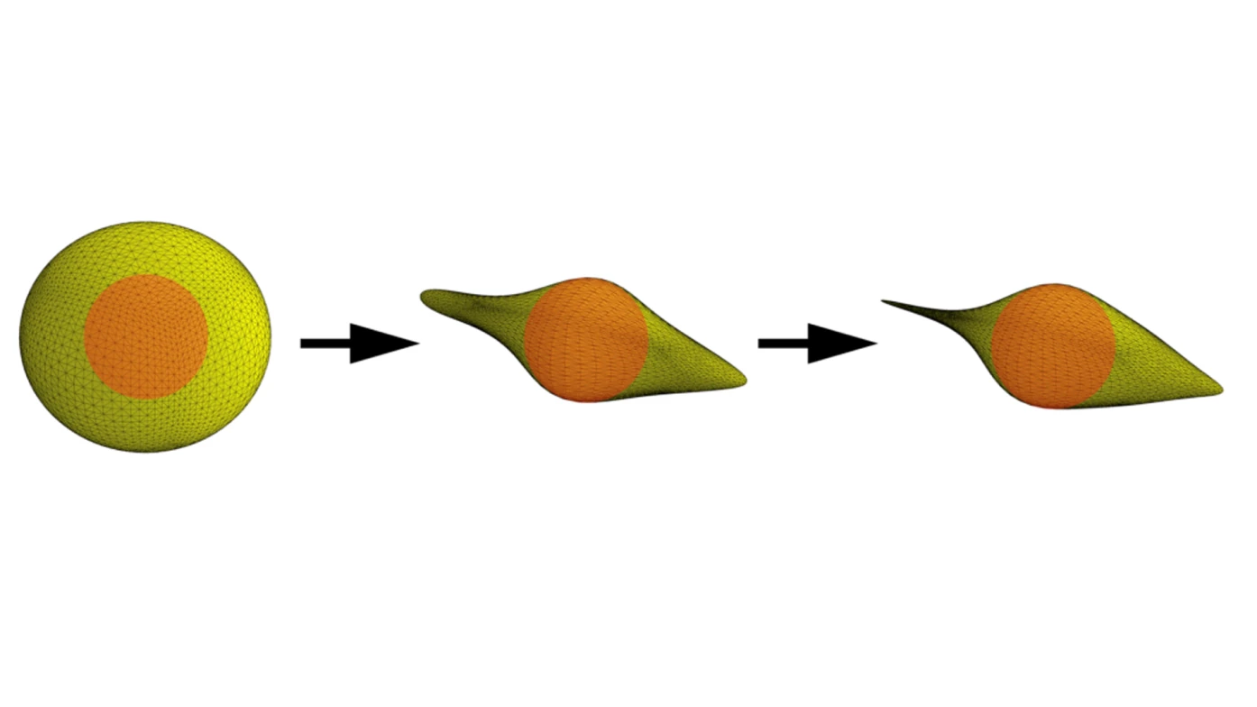
What does optimizing a shape mean? The below figure is a simple example of aerodynamic optimization. Geodesic convolutional shape optimization means changing the shape with algorithms that are not explicitly programmed to create a certain shape. Rather, using deep learning techniques, the algorithms compare the objective it has been given (e.g. minimise the airflow resistance) with the shape it modifies and check with a simulation, not taken from external software but from its learning based on experimental or CFD data. Although elementary in shape, the example fully shows how training and testing data from existing computational fluid dynamics datasets can create an ideal streamlined shape, starting from a spherical surface and without intermediate steps from humans.

Researchers at EPFL (Lausanne, Switzerland) and Neural Concept introduced a new type of deep convolutional neural network able to compute convolutions efficiently over a geodesic surface described by a mesh.

The Computer Vision Lab of EPFL (Lausanne, Switzerland) and Neural Concept have been active in the field of application of geodesic convolutional shape optimization from the early beginnings indeed, with a seminal publication at the 35th International Conference on Machine Learning, 10-15 July 2018, Stockholmsmässan, Stockholm (Link to Video).

This is a very early application of deep learning to aerodynamic shape optimization, considering that it was, in general, unknown to the public of engineers until 2012 at least, and the first applications were related to relatively more straightforward 2D image recognition and other “Euclidean” application such as text and audio recognition.

They trained such a Geodesic Convolutional Neural Network to predict the aerodynamic performance measure of interest (e.g. CX, drag, lift). Then, they used this gCNN predictor as a differentiable black-box surrogate model mapping a shape design to an objective. Using techniques originating from computer vision, the team optimized the shape given as input to this surrogate with a gradient-based technique, resulting in a new optimization method, non-parametric and able to take into account additional shape constraints in a very flexible way.

Experimental validation on 2D and 3D aerodynamic shape optimization problems demonstrated that it makes optimization possible for large parameter spaces where previous approaches failed.

The simple example of geometric deep learning can be extended to more complex shapes, thus envisaging full car aerodynamic shape optimization. Training and validation data can be obtained from departments such as methodology, CAE and R&D, which store hundreds or maybe thousands of cases per year for automotive and aerospace organizations. This has even led to pre-trained models for turbomachines where users (or algorithms) can access multiple prediction points.

Comparison of Traditional and AI-Based Product Design Cycles

We will first introduce typical practices in the traditional product design cycle and then compare those practices with the proposed workflow of performing shape optimization with computer vision techniques.

The Traditional Product Design Cycle

The traditional product design cycle is an iterative process that involves several stages to develop a product from concept to final product. The stages include initial design (1), simulation to check the shape’s behaviour from an engineering point of view and verify if functional objectives are met (2) and finally, redesigning (3) until the functional objectives are met. Let us detail the three stages.

Stage 1: Design a Shape

This is the initial stage of the product design cycle, where the product designer creates a conceptual design of the product. They use various tools such as sketches, Computer-Aided Design (CAD) software, and 3D modelling to represent the product visually. Also, methods more similar to computer vision, such as CAS (computer-aided styling or computer-aided industrial design), are used early in the concept phase.

Stage 2: Simulate the Shape’s Behaviour

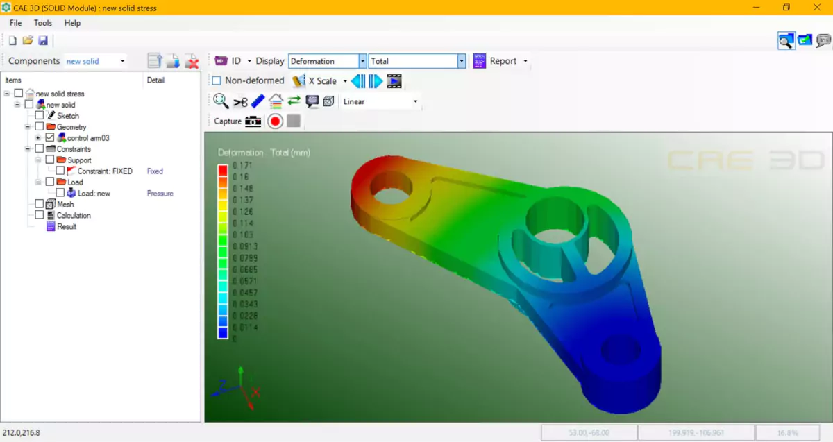
Once the initial design is created, the designer simulates the product’s performance using computer simulations. This includes analysing the product’s stress and strain, thermal and fluid behaviour with FEA and CFD. This step helps the designer identify any potential issues with the design and make necessary adjustments.

Stage 3: Redesign the Shape

Based on the simulation results, the designer may need to make changes to the design. This can include modifying the design’s shape, materials, or other aspects to improve the product’s performance. The redesign process is repeated until the product meets all the requirements and specifications.

Design Cycle Based on Objective Function and Deep Learning: Shape Optimization Pipeline

The design cycle based on an objective function and deep learning is a new approach to product design that utilises advanced optimization techniques and machine learning algorithms. The optimization pipeline is a process that combines traditional design methods with cutting-edge technology to create highly optimized and functional products.

The first step in the pipeline is to define an objective function (OF).

Objective Function (OF)

An OF is a mathematical expression representing the product's design goals- generally reaching a maximum or a minimum for one or more variables “x”. Also, keeping a value of a variable x at a certain level X means to make the difference between x and X minimum. For example, an OF for a car design may include minimising weight while maximising fuel efficiency.

The objective function is the foundation for the entire design process and guides the optimization process. Once the OF is defined, the next step is to use deep learning algorithms to optimize the product’s shape.

Enter Deep Learning in the Pipeline

Deep learning algorithms, such as convolutional neural networks and supervised learning, are taken from computer vision methodologies. They analyse and optimize the product’s shape based on the OF. These algorithms can quickly evaluate millions of different design options and identify the optimal shape for the product.

Enter Simulation in the Pipeline

The optimization pipeline also includes a simulation step where the optimized shape is simulated to evaluate its performance. This step is critical to ensure that the product meets all the design requirements and specifications. The simulation step also helps identify potential design issues and make necessary adjustments.

Where Design Is Happening: Shape Space (Design Space)

Where is the arena where all the operations described in this article occur? It is a very important one in an industrial process, upstream of manufacturing and delivery. We will first describe the scenario before the advent of AI and advanced techniques such as convolutional neural networks.

The promise of Industry 4.0 was to have, for a physical object (a delivered product or a machine producing it), a physical twin representing it digitally. How to ensure that the product or machinery satisfies the requirements (targets and constraints), such as being efficient or powerful or durable and sustainable? Because the product design department of the manufacturer found an optimal, or a relatively best solution, with digital tools such as CAD (for shape modelling) and CAE (for checking the shape behaviour). To explore the range of designs created from a given set of targets and constraints, designers move within the “design space”.

A Design Space is a mathematical concept that refers to the set of all possible designs that can be generated from a particular set of design parameters.

In aerodynamics wing shape optimization, for example, the Design Space could be defined as the set of all possible wing shapes created from a given set of design parameters such as wing span, chord length, and airfoil shape. Engineers use computational fluid dynamics (CFD) simulations to explore the shape space and find the wing shape that will provide the best performance for a given set of constraints, such as lift-to-drag ratio, stall angle, and maximum lift coefficient.

In car shape optimization, there could be a specific shape space for side mirrors and another shape space for spoilers, each with a set of very specific constraints and objectives - for instance, this spoiler shape space is less constrained for aeroacoustics than mirrors. In contrast, mirrors are less constrained for downforce.

Engineers can use mathematical techniques such as optimization algorithms to search the Design Space and find the best design.

Methodology and Definitions - What Is the New Deep Learning Approach? Optimizing Without Shape Parameters

We will review here, starting from elementary concepts, how deep learning can speed up computations to provide a quasi-real-time alternative to extremely computationally demanding methods.

Supervised Learning - an Elementary Explanation

Let's imagine that, as AI experts, we were invited to our children’s school to explain what are Mum or Dad doing. The naive explanation could run as follows:

“Supervised learning is a way for computers to learn stuff by being shown many examples. It’s like your teacher giving you many math problems to solve and then checking the answers to see if they are correct. This way, you will learn how to solve similar problems independently. Supervised deep learning is similar, but instead of math problems, the computer is shown many examples of something, like pictures of cats and dogs. It then uses those examples to learn how to recognise new pictures of animals. The same can be done with other objects, such as cars, trucks, vans or bicycles.

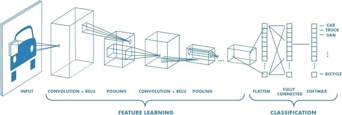
In other words, the computer is given a set of labelled examples (input data and the expected output), and it uses that data to learn a function that maps the input to the output. Then, the computer can use this learned function to make predictions on new, unseen input data. So, supervised deep learning is a way for a computer to learn from examples, with the help of labelled data, and make predictions on new, unseen data.”

Supervised Deep Learning - an Advanced Explanation

Once we have given the naive explanation, let us see what is seriously behind it in the language of mathematics.

From the previous section, we have understood that we will implement a method in which a deep neural network is trained to map inputs to outputs using a dataset.

Therefore, we want the deep learning algorithm to find a function f=f_θ(x) that connects inputs x and outputs f. The training process involves minimising a loss function L(y,f_θ(x)), which measures the difference between the network’s predicted output f=f_θ(x) and the true output y for a given input x.

Formally,

• let x be an input
• let y be the corresponding true output
• let f_θ(x) be the predicted output of the neural network parameterised by θ.

The loss function L(y,f_θ(x)) is defined to measure the difference between the predicted and true output. The objective of the training is to find the parameters θ of the neural network that minimises the expected value of the loss function over the training dataset, that is:

θ^ = argmin_θ (1/n) * Σ_{i=1}^n L(y_i,f_θ(x_i))

where n is the number of samples of the training dataset.

Once the neural network is trained and its parameters θ are optimized, it is tested. Once tested, it can make predictions on new, unseen input data. The predictions are made by forwarding the input through the trained neural network, which produces an output based on the learned mapping. This is a “predictive model”.

The accuracy of the model predictions can be evaluated by comparing them to the true output for a given input during the testing phase. In supervised learning, the training set and testing set are used to evaluate the performance of a model. 

• The training set uses its full knowledge of the accessible portion of the dataset to train the predictive model. 
• The testing set evaluates the trained model performance on unseen data, i.e. they are accessible only to humans.

The percentage of the data allocated to the training set and the testing set can vary based on the dataset size and the specific application. However, there are some general guidelines for the proportion of the data that should be allocated to each set.

• One common practice is allocating 80% of the data to the training set and 20% to the testing set. This is a good starting point for many applications, as it provides a large enough training set to allow the model to learn the underlying patterns in the data while providing a sufficient testing set to evaluate its performance.
• Another approach is to use a more balanced split, such as 70% for training and 30% for testing. This is useful when the dataset is small, and the model is expected to be more sensitive to the size of the training set.

It is important, during training, to avoid overfitting. Overfitting in neural network training occurs when a model performs too well on training data and cannot generalize to new, unseen data. One of the ways overfitting can happen is if a model is trained on a small dataset and has too much capacity to fit the noise in the data rather than the underlying pattern. There are several techniques to avoid overfitting. Regularization techniques, like L1 and L2, are an example.

• L1, also known as Lasso regularization, has a term proportional to the (absolute) value of the weights. As a result, some weights are shrunk towards zero, effectively removing them from the model. This can be useful for feature selection as it can help identify the most important features for the model’s predictions.
• L2, also known as Ridge regularization, has a term proportional to the weights’ square. This results in all weights being shrunk, but not necessarily towards zero. This can help to improve the stability of the model and reduce overfitting.

Other techniques are early stopping, dropout, and of course, using more data.

Methodology and Definitions - What Is a Convolutional Neural Network?

“Convolutional” in CNN stands for “convolutional neural network.” A convolutional neural network is an algorithm commonly used for image recognition and other tasks involving image-like data, such as natural language processing. The convolution operation is used to extract features from the input data. In the case of images, convolution is used to identify patterns and features such as edges, textures, and shapes.

In convolutional neural networks, the input data is passed through multiple layers of convolutional filters. Each filter performs a convolution operation on the data. These filters are trained to recognise specific features in the input data. More complex features are extracted as the data passes through the filters’ layers. This process is called feature extraction.

The extracted features are then passed through multiple layers of artificial neurons, also known as fully connected layers, to classify the input data. The last layer of neurons is used to generate the final output of the model. In the image below, An atrous geo conv block is a specific building block used in deep learning models that combine the “atrous convolution” and “geodesic convolution” techniques. Atrous convolution is a technique used in convolutional neural networks to increase the receptive field of filters without increasing the number of parameters.

The shown techniques learn features from the input data that are invariant to the geometric transformations and capture the multi-scale information of the input data.

Methodology and Definitions - What Is a Geodesic Convolutional Neural Network?

A regular CNN is designed to work on data defined in a Euclidean space, such as images or text. However, some data, such as 3D shapes, are defined on non-Euclidean manifolds. Geodesic Convolutional Neural Networks are designed to handle this kind of data by incorporating the geometric information of the input data into the network. Geometric information of the input data is incorporated into the neural network by performing the convolution operation along the geodesic paths of the input data’s manifold. This allows the convolutional neural network to take into account the intrinsic geometric structure of the data, making it suitable for handling data that is defined on non-Euclidean manifolds.

The main difference between a regular CNN and a geodesic CNN is how the convolution operation is performed.

• In regular Convolutional Neural Networks, the convolution operation is performed by sliding a filter over the input data.
• In geodesic Convolutional Neural Networks, the convolution operation is performed by sliding the filter along the geodesic paths of the input data’s manifold. This allows the network to consider the data’s intrinsic geometric structure.

Geodesic CNNs have been used for various tasks, such as 3D shape classification, surface parameterization, and 3D object detection. Geodesic convolutional neural networks have also been used in medical imaging, computer vision, and robotics applications, where the input data is defined on non-Euclidean manifolds.

Why CCNs Are Better than Artificial Neural Networks

A fully connected artificial neural network (FC-ANN) and a convolutional neural network (CNN) are different architectures with different capabilities.

• An FC-ANN is a feedforward neural network where each neuron in one layer is connected to every neuron in the next layer. FC-ANNs are commonly used for tasks such as classification and regression and can be trained to recognize patterns in the input data.
• On the other hand, a CNN is specifically designed for image recognition tasks. It uses convolutional layers consisting of filters that move across the image and extract features at different spatial locations. Filters are trained to recognize specific features such as edges, textures, and shapes in the image. CNNs also use pooling layers which reduce the input's spatial dimensions and help reduce the number of parameters in the network. We will see more of this before this article's conclusion regarding computational performance.

Since associating a surrogate of a CFD or FEA result to a CAD is a sort of image recognition process, it becomes clear why CNNs and not FC-ANNs are the only industry-grade solution.

How Are Shapes Modified?

RBF is a technique that can be used to interpolate or approximate a function from a set of data points. Given a set of data points (x₁, y₁), (x₂, y₂),...,(xₙ, yₙ), and a set of control points (c₁, c₂),...,(cₘ, cₙ), RBF can be used to approximate the function f(x) that fits the data points by minimising the following OF:

f(x) = Σᵢ wᵢ * φ(||x-cᵢ||)

where Σᵢ is a sum from 1 to N; wᵢ are weights; cᵢ are control points; φ(||x-cᵢ||) is a radial basis function (RBF); and ||x-cᵢ|| is the Euclidean distance between x and cᵢ

In geometry morphing, the control points are used to define the shape of the geometry, and the RBF interpolates the shape between the control points. The weights can be optimized to create smooth transitions between different shapes, creating a smooth and continuous change in the geometry.

Benchmarking AI Algorithms - The Kriging Method

Kriging is a valuable method for mining and oil and gas exploration businesses. It is named after the venerable mining engineer and statistician South African Danie Krige, who lived from 1917 until 2013 (just at the dawn of the Deep Learning era). Krige’s seminal work is “A statistical approach to some basic mine valuation problems on the Witwatersrand” (full reference in the Appendix). Kriging is a method that estimates the value of a variable at a location based on measurements taken in nearby locations. Kriging uses statistical models to predict the value of a variable at a point based on the values of that variable at nearby points.

Kriging Usage

Kriging is a linear interpolation method that minimises the mean square error of the estimates. It is based on a stochastic process (a mathematical model describing a variable’s behaviour over space and time). The key assumption in Kriging is that the variable of interest is the realization of a stationary stochastic process characterised by a function, also known as the “variogram”. The variogram is a covariance: in practice, it describes the degree of spatial dependence between two locations in the field. Let’s dive into some mathematical details in the below section. If you want to grasp how Kriging compares to CNNs, you may skip the next section and go to “Four Basic Reasons Why Kriging Is Not Performing Like CNNs”.

The Mathematics of Kriging

Kriging estimate of the variable z at an unsampled location, z₀, is given by:

z₀ = Σᵢ(wᵢ * zᵢ)

where Σᵢ is the summation of the i’s and the weights wi are determined by solving a system of equations (j is the summation of the j’s);

Σⱼ (wᵢ * C(zᵢ, zⱼ)) = C(z₀, zⱼ)

• C(zᵢ,zⱼ) expresses the covariance between the observations zᵢ and zj at locations i and j,
• C(z₀,zⱼ) expresses the covariance between the unsampled location z₀ and the jth observation zⱼ.

4 Reasons Why Kriging Is Not Performing Like CNNs

Kriging is excellent in many practical applications in mining or prospection for oil and gas but less so for product design in industries such as Automotive, Aerospace, Electronics, Machinery, Shipbuilding or Medical Devices; in such a case, it has several disadvantages compared to (geodesic) convolutional neural networks or (g)CNNs.

1. More complex: Kriging requires significant computational resources to estimate the variogram, determine the weights, and make predictions. CCNs, on the other hand, are neural network-based models that can be trained and used for prediction with significantly fewer computational resources.
2. Less flexible: Kriging is based on the assumption that the underlying process is stationary (and isotropic) - which may not always be the case! CCNs are not based on assumptions about the underlying process and can be used for many problems and data types; hence, CNNs are more generalizable.
3. Less ability to handle nonlinearity: Kriging is a linear interpolation method unsuited for handling nonlinear relationships in the data. CCNs, being neural networks, can model nonlinear relationships. It does represent a major advantage of CNNs over Kriging.
4. Less ability to handle large-scale datasets: Kriging is relatively less well-suited to handle large-scale datasets due to the computational complexity and limitations of the method. GCNNs, on the other hand, are well-suited to handle large-scale datasets and can be trained on high-dimensional data.

How is Kriging Implemented to Car Aerodynamics?

For fairness, we describe how to approach an aerodynamics problem with Kriging. It’s important to note that, as shown in the previous section, Kriging has some limitations regarding non-linearity and high-dimensional data, and it may not be the best method to model the aerodynamics of a car! Therefore, it’s important to consider other methods, such as CCNs or machine learning models, which can handle non-linearity and high-dimensional data better. Implementing Kriging for car aerodynamics would involve several steps:

1. Collect the Data. The first step would be to collect data on the variable of interest, such as air resistance or drag coefficient, at various locations on the car’s surface. This data can be collected through wind tunnel testing or computational fluid dynamics (CFD) simulations.
2. Estimate the Variogram. Once the data has been collected from the previous passage, the next step would be to estimate the variogram, which describes the spatial correlation structure of the variable of interest. This can be done using experimental variogram techniques, such as the semivariogram or the Kriging variogram.
3. Data Interpolation. Using the estimated variogram from the previous passage, Kriging can then interpolate the variable of interest at unsampled locations on the car’s surface. The weights for each sample are computed using the estimated variogram and solving the system of equations.
4. Predictions. With the interpolated data, Kriging can predict the variable of interest at any location on the car’s surface. These predictions can optimise the car’s aerodynamics and reduce air resistance or drag.

Finally, it is important to validate the predictions made by Kriging by comparing them to measured data. This can be done by comparing the predictions to wind tunnel or CFD results at the same locations.

Benchmarking Shape Optimization Algorithms

We will review and compare three methods that have been implemented and are still popular in optimization. This will allow benchmarking optimization algorithms.

Genetic Algorithms (GA)

‍GAs are a diffused and relatively easy-to-implement approach where shape optimization relies on genetic algorithms, i.e. optimization techniques inspired by natural selection. GAs create a population of candidate solutions and evaluate their fitness according to a “fitness function”. Then, genetic operators (such as “crossover” and “mutation”) are iteratively applied. This will make the population evolve towards better solutions.

GAs are good at finding global solutions in large, complex search spaces. However, GAs can be computationally expensive, especially for high-dimensional problems. Additionally, GAs can be sensitive to the choice of the initial population and the genetic operators used. This can affect the quality of the final solution.‍

Adjoint differentiation

Adjoint differentiation is a technique for efficiently computing the gradients of an OF. Gradients are computed on the design variables. The adjoint method is based on the idea of solving an adjoint equation that is related to the original forward equation. Adjoint differentiation can be highly efficient for large-scale optimization problems. It can handle both linear and nonlinear problems.

However, adjoint differentiation requires the ability to solve the adjoint equation. This can be computationally expensive and have difficulties dealing with constraints and non-differentiable functions.

More on the adjoint method. The adjoint method is used in numerical analysis to solve partial differential equations (PDEs). It is based on the idea of introducing an adjoint equation that is related to the original forward equation. The adjoint equation is a PDE derived from the original equation by taking the transpose of the equation and reversing the direction of time or space.
An example of the adjoint method can be seen in the heat equation, which is a PDE describing heat distribution in a solid object. The “forward” (physical space) equation for the heat equation is: ∂u/∂t = α ∇²u, where: u is the temperature distribution in space and time, t is time, and α is the thermal diffusivity of the solid object. The operators are the following: ∂/∂t is the time time, ∇ is the gradient (space derivative) symbol, and ∇² is the Laplace operator.

For those not into heat transfer, this equation is intuitive. For example, an object with large diffusivity α will heat up faster (larger ∂u/∂t) than an object with smaller diffusivity α (N.B. all the rest being equal!). Now, to derive the adjoint equation, we take the forward equation’s transpose and reverse the time’s direction: ∂u*/∂t* = -α ∇²u*, where: u* is the adjoint variable, and t* is the reversed time.

Bayesian Optimization with Surrogates‍

Bayesian optimization is a technique that uses a probabilistic model to predict the performance of candidate solutions and guide the search towards promising areas of the design space. Surrogate models approximate the OF, reducing the number of function evaluations required to converge to an optimal solution. This approach is particularly useful when the OF is expensive to evaluate. However, it can be computationally expensive for high-dimensional problems. Also, it can be sensitive to the choice of the surrogate model. This can affect the quality of the final solution.

Short note for those unfamiliar with probability theory: "Bayesian" in "Bayesian Optimization" refers to using Bayesian probability theory in the optimization process. In Bayesian probability theory, probabilities are represented by probability distributions rather than just single values. This allows for the incorporation of prior knowledge and uncertainty into the analysis. In Bayesian optimization, the optimized objective function is treated as a random variable with a probability distribution. This distribution is updated as new data is acquired, and the optimization algorithm uses this information to guide the search towards the optimal solution.

Case Study: NACA Profiles and their Optimization

Let's introduce NACA profiles for those unfamiliar with aerospace engineering.

NACA profiles are airfoils developed by the National Advisory Committee for Aeronautics (NACA) in the United States during the 1930s. They are known for their simple and easy-to-construct shapes and their good performance at low speeds.

The NACA airfoils are defined by a four-digit number code representing the airfoil’s shape.

• The first digit represents the camber (i.e., the curved shape of the upper surface of the airfoil)
• the second digit represents the position of the maximum camber
• the third and fourth digits represent the thickness distribution of the airfoil.

Interestingly for deep learning, there are datasets of CFD computations of NACA profiles. These datasets typically include the results of simulations of the flow around NACA airfoils at different angles of attack, Reynolds numbers, and Mach numbers. They can include data such as lift and drag coefficients, pressure distributions, and flow velocities.

Some datasets are publicly available; for example, NASA has a dataset built with CFD computations of NACA airfoils, which includes the results of simulations of the flow around different NACA airfoils at different angles of attack and Reynolds numbers.

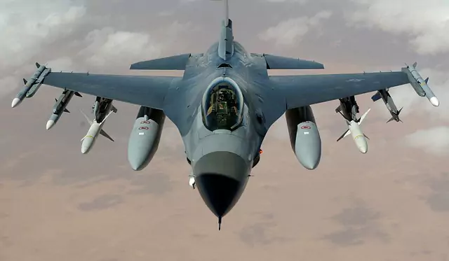
What are the objectives for the geodesic convolutional shape optimization of an airfoil? Let's start in 2D. Here we want to maximise the aerodynamic lift (vertical upwards force) with low drag. The key ingredients are in-the-loop shape modification and the predicting aerodynamic quantities, such as pressure, driven by the optimization algorithm. Here, shape deformations were performed by each vertex in the profile moving independently, and the obtained profile confirms known results in the literature.

Shape Change for Large Meshes

The previous method may be computationally intensive in the case of a large set of vertices representing the shape. Rather, a representation of the latent parameters of a shape is sought.

In the case of NACA profiles, there are standard industry parameterizations. The case shown here illustrates the seek for more aerodynamic lift Cl (left to right in the below figure) while also having more pitching moment Cm (from top to bottom in the below figure).

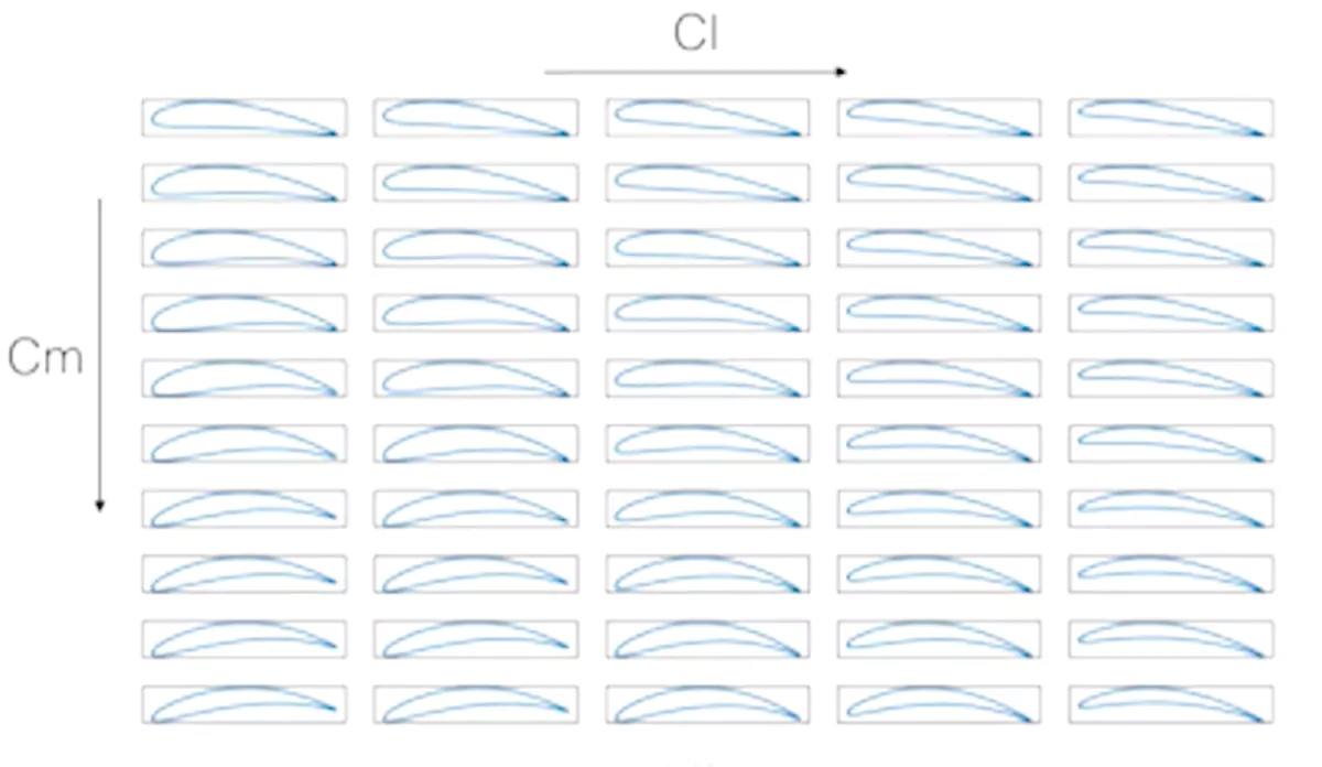
Again, AI, based only on data and learning algorithms, rediscovers the consolidated knowledge that changing the angle of attack is beneficial for the lift while changing the curvature influences the pitching moment. Also, shape constraints can be imposed. This has great relevance when designing industrial shapes. Taking the 2D profile again but developing it in 3D, we could impose that the shape change process should preserve an internal sphere. The video shows a neural network with full 3D optimization capabilities.

The point about the above experiments is to be able to move on to shapes where there is no consolidated body of knowledge, i.e. designing shapes in an industrial context with variable objectives and constraints and the ability to leverage training data produced by the R&D or CAE offices.

There are several more cases, such as UAV design optimization with the support of an extensively documented white paper.

Case Study: Hydrofoils and Their Optimization

Hydrofoils are wing-like structures attached to a boat’s hull and are designed to lift the boat’s hull out of the water level. This is important at high speeds.

Since air will resist less than water, hydrofoils can significantly reduce drag and increase the speed and efficiency of the boat. Hydrofoils are commonly used in marine racing, particularly in high-speed boats such as hydroplanes and catamarans.

In hydroplane racing, the hydrofoils are attached to the bottom of the boat’s hull and lift the hull out of the water at high speeds, allowing the boat to “fly” above the water’s surface. This reduces drag and increases speed, allowing the boat to travel faster than it would with just the hull in the water.

In catamaran racing, the hydrofoils are attached to the sides of the boat’s hulls and lift the hulls out of the water at high speeds. This reduces drag and increases speed, allowing the boat to travel faster than it would with just the hulls in the water.

BMW Oracle Racing, an American sailing team, won the 33rd America’s Cup in 2010 against the Swiss team Alinghi. America’s Cup is considered the oldest international sports trophy and is awarded to the winner of a sailing race. Eventually, the two teams agreed to race in giant trimaran yachts with a 90-foot wing sail. BMW Oracle Racing’s trimaran featured a unique design, with a rigid wing sail that was more than twice the size of the sails used on traditional America’s Cup yachts. This unique design gave BMW Oracle Racing a significant performance advantage over the Alinghi team. The final race took place on 14 February 2010 in Valencia. BMW Oracle Racing’s trimaran (USA 17) sailed to a 2'22" victory over Alinghi 5. This victory marked the first time in the history of the America’s Cup that a multihull boat won a trophy.

Optimizing the hydrodynamics properties of hydrofoils is now key to designing their shapes. However, it remains very challenging because actual Computational Fluid Dynamics techniques rely on solving Navier-Stokes equations, and this has to be performed for every different shape. This is computationally demanding but also quite restrictive. Indeed, with classical CFD techniques, the changes in geometries are limited, as only a few designs can be tested before reaching a final geometry. Those limitations were the main reasons and motivations for this project. As it will be shown, more complex geometries can now be tested as multiple degrees of freedom can be changed at the same time, and it is possible to fine-tune each of the geometrical parameters.

In this study, the authors applied a numerical optimization method for Hydrofoil shapes on EPFL’s Hydrocontest race boat. We show that the numerical optimization method based on Geodesic Convolutional Neural Network techniques (Baqué et al., ICML 2018) improves the foil’s design upon previously manually optimised shape. The authors first demonstrated the potential of this approach on the simpler 2D hydrofoil profile optimization using the XFoil CFD solver. We then extend this method to optimize the full 3D shape using MachUpPro, an advanced non-dimensional lifting surface analysis code.

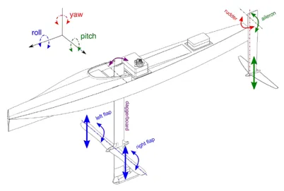
The algorithm allowed a calculation time of around 1 to 2 minutes for a full simulation, whereas it is within the scale of hours for the previous physics-based solvers. The versatility to adapt to any geometry was also a major advantage.

Closing Questions: Does Deep Learning Speed Up the Computation? And How?

We have seen that a neural network can be trained to approximate the solution to an aerodynamics problem. Also, it can be a full surrogate of the whole CAD reading - CAE output process if solutions like NC Shape, based on geodesic CNNs, are used.

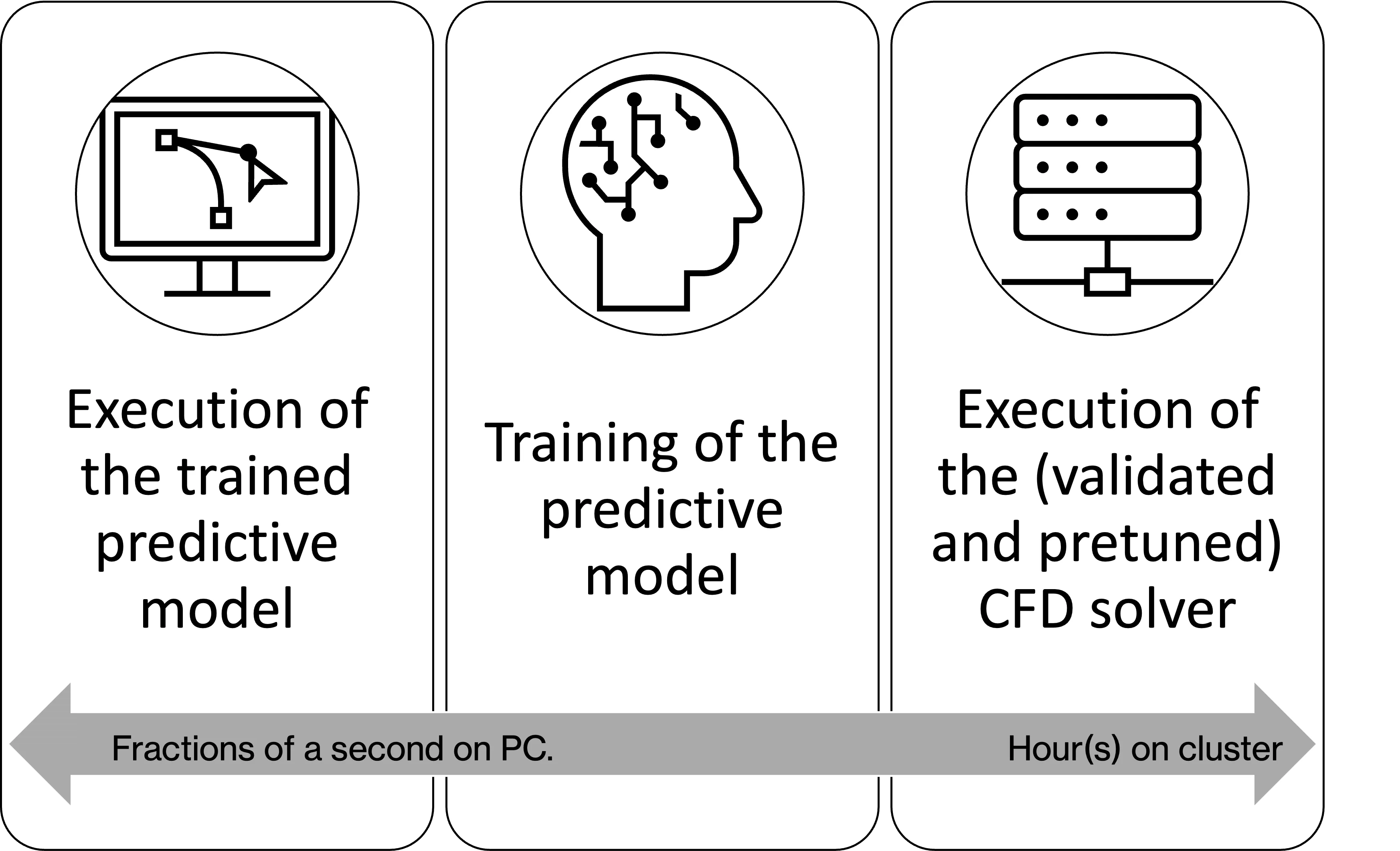
The training phase for a neural network can be computationally expensive, but once trained, the neural network can make predictions relatively quickly. Once trained, it can predict the solution (pressure, velocity and other fields) much faster than a traditional CFD simulation. For example, a simulation taking 3 hours on 32 CPU cores can be accelerated up to 0.3 seconds on a single core. The investment required to train the network could be around 6-8 hours on a dedicated GPU.

In "Big O" notation (disclaimer - the following is the author's guesswork without claims of deep research work):

• The time complexity of computational fluid dynamics (CFD) simulations is generally considered (in big O notation) O(n³) or higher, where n is the number of grid points or cells used in the simulation. This is because CFD simulations typically involve solving partial differential equations (PDEs) on a grid, which can be computationally intensive.
• The time complexity of neural network training, the time complexity is typically measured by the number of iterations, or epochs, required to train the network and the time it takes to perform each iteration. The time complexity of each iteration is determined by the number of parameters in the network, which is related by factors such as the number of layers and the number of neurons in each layer. The time complexity of training a deep learning model is often O(n), where n is the number of parameters in the network.
• CNNs introduce speed-up compared to traditional neural networks thanks to Filters and Pooling.
• Filters are a technique to extract features from the input image. Filters are typically small matrices moved across the image, performing a dot product (between matrices) with the local image patch at each location. The outcome of the dot product reduces the number of parameters in the network. It can also reduce the spatial dimensions of the input, which can help reduce the network's time complexity.
• Pooling is a technique used to reduce the spatial dimensions of the input in a CNN. It is typically applied after the convolutional layers and works by down-sampling the input image taking the maximum or average value of a small window of pixels. This process reduces the number of parameters in the network and can also reduce the spatial dimensions of the input, again reducing the network's time complexity.
• The time complexity of trained neural network execution (i.e. once trained) could be O(log n), where n is the number of parameters in the network. This is because the forward-propagation step, used to make predictions, typically involves a series of operations, such as activations that can be done in parallel and are relatively fast. We can say that a neural network execution for a modern gCNN is roughly the same magnitude of being real-time (0.02 to 1 second for most Neural Concept use cases).

Summary

We have shown how a computer vision-inspired approach can improve efficiency in the product design departments by empowering drag and pressure prediction in aerodynamics and moving forward with optimization. We also have seen traditional methods like Kriging and what is the added value provided by convolutional neural networks. More specifically, we have seen how geodesic convolutional networks act and how they can support convolutional shape optimization for 2D and 3D cases. We have estimated the speed of execution of trained neural networks, thus making it feasible to conceive fast optimization loops exploring such methods as the gradient-based technique both for neural network training and shape optimization, exploiting differentiability properties. Being data-driven, neural information processing systems can move in a large shape space, starting from an initial shape and finding a feasible shape within maybe previously unseen shapes. This new surrogate model method is a surrogate for CAE and, coupled with a gradient-based technique, provides a fully closed-loop solution with the potential to manage shapes of arbitrary complexity.

Next Steps

What is the "evolution" to expect concerning the material shown so far? We want to highlight at least four tracks.

1. CAD-PLM integration: Tighter integration to CAD formats, such as native files
2. Pre-trained models: Availability of pre-trained models for specific applications to accelerate the adoption process in organizations that have not yet reached sufficient maturity in building their datasets or need casual usage without investing in the preliminary CFD CAE technology
3. Data Fusion: Multiple-level integration of CFD, solid mechanics and electromagnetic data coming from industry-grade, high-fidelity R&D grade and experimental data
4. Uncertainty Estimation: When modifying a shape, the predictor could enter a zone of the shape space with never seen configurations. Rather than going forward with predictions, it could be useful to estimate the confidence in the prediction and, when needed, call back the ground truth to have a few more predictions to calibrate the predictor in the new zone of the design space.

Please note that the above points are not Neural Concept plans; they are all already implementable, and their implementation depends on the business case for the user.

For example:

1. CAD-PLM integration is of particular interest to product engineering departments.
2. Pre-trained models could be an interesting case for companies who need to optimize the size of training datasets.
3. Data Fusion could be very appealing for companies with multiple data sources, e.g. for the manager of a Wind Tunnel with a group of CFD analysts who would wish to exploit both 40 years of wind tunnel data and 20 years of CFD data.
4. Uncertainty Estimation is important for reliable predictions during optimization processes to have a validated final industrial shape.

Appendices

The XFoil CFD Solver

XFoil is a Computational Fluid Dynamics (CFD) solver specifically designed to analyse airfoils, which are the cross-sectional shapes of wings or blades. XFoil is a 2D panel method solver, which means it solves the flow around an airfoil by dividing the surface of the airfoil into a series of small, flat panels and then solving the flow equations at each panel. XFoil uses the Navier-Stokes equations to model the flow around the airfoil, a set of equations describing the fluid flow’s behaviour. The Navier-Stokes equations are solved using various methods, such as the panel method, which models the flow as a series of flat panels, or the vortex lattice method, which models the flow using a series of vortices. XFoil is known for its ability to accurately predict the aerodynamic performance of airfoils, including lift, drag, and stall characteristics, under a wide range of conditions, including subsonic and supersonic flows, and at different angles of attack and different Reynolds numbers. XFoil can analyse existing airfoils’ performance and design new airfoils with specific performance characteristics.

Bibliography - Basic Reference on gCCNs and Optimization

The following article is seminal. Since its publication, Neural Concept has introduced many more techniques and practical features for NCS users!

"Geodesic Convolutional Shape Optimization" by Pierre Baqué, Edoardo Remelli, François Fleuret, Pascal Fua (ref. arXiv:1802.04016)

Summary: Aerodynamic shape optimization has many industrial applications. Existing methods, however, are so computationally demanding that typical engineering practices are to either try a limited number of hand-designed shapes or restrict oneself to shapes that can be parameterised using only a few degrees of freedom. This work introduces a new way to optimise complex shapes quickly and accurately. To this end, the Authors train Geodesic Convolutional Neural Networks to emulate a fluid dynamics simulator. The key to making this approach practical is re-meshing the original shape using a polycube map, which makes it possible to perform the computations on GPUs instead of CPUs. The neural net is then used to formulate an objective function differentiable with respect to the shape parameters, which can then be optimised using a gradient-based technique. This outperforms state-of-the-art methods by 5 to 20% for standard problems, and even more importantly, the approach applies to cases that previous methods cannot handle.

Bibliography - Basic Reference on Kriging

The following article is the foundation of Kriging: “A statistical approach to some basic mine valuation problems on the Witwatersrand”, Danie G. Krige, J. of the Chem., Metal. and Mining Soc. of South Africa. 52 (6): 119–139 (December 1951)

‍