Drone Aerodynamics — Design Optimization by SenseFly & NC

Optimizing the shapes of unmanned aerial vehicles is crucial for improving flight performance. Engineers can efficiently optimize drone designs using multiple levels of simulation fidelity, allowing drones to fly longer and maintain stable flight maneuvers. The solution combines the Neural Concept platformwith AirShaper's cloud-based aerodynamics simulations. The innovative role of AI in aerospace engineering is shown during the initial concept phase.
1 Introduction - Optimizing Drone Flight
Optimizing the shape of unmanned aerial vehicles is of primary importance for the industry. SenseFly, one of the market leaders in the fixed-wing drone segment, is always looking to minimize the battery consumption of its aircraft and, therefore, make drones fly longer. Since aerodynamic design directly influences in-flight performances, slight improvements are important, bringing a non-negligible technological lead over competition in the drone technology arena.
Numerical simulations can assess the flight performance over a range of flow velocities and flight conditions before building the drone. Nevertheless, these simulations are numerically expensive. Therefore, multiple levels of fidelity are used. A rule of thumb is that the lower the simulation fidelity, the quicker and less expensive the result.
The AirShaper platform empowers engineers with drone aerodynamics simulation in the cloud, starting from their uploaded 3D models. However, a campaign of aerodynamic optimization remains tedious and time-consuming, even with a very efficient and reliable numerical simulation platform.
This report shows how the Neural Concept optimization platform can be combined with AirShaper and exploit multiple fidelities to reach an optimal design quickly.
1.1 Drone Flight - Basic Principles on How Drones Fly
How do drones fly? Drone flight involves a combination of various forces that enable stable and efficient flight.
Drones fly efficiently when they can generate sufficient thrust, control angular velocity, and optimize aerodynamic performance. These factors collectively enable drones to reduce drag, maintain stability, and achieve the desired flight efficiency for applications like package delivery.
A critical aspect of tasks such as package delivery is the generation and management of thrust. Thrust propels the drone forward, overcoming drag (the aerodynamic resistance encountered as the drone moves through the air). Efficient thrust is essential to reducing drag and maintaining optimal aerodynamic performance.
Drones utilize control surfaces that adjust angular velocity (the rotation rate around the drone's axes) to achieve flight stability. By precisely controlling it, drones can maintain their position or change direction.
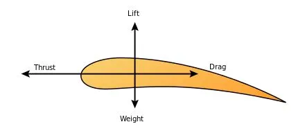
Stable flight and flight maneuvers under control require a balance of forces: lift (upward force), weight, thrust by the propulsion system, and drag (air resistance), as shown in Figure (1).
Lift is the force that counteracts the drone's weight, allowing it to ascend and stay aloft. Control surfaces adjust the drone's orientation and direction by manipulating its airflow.
The lift-to-drag ratio L/D is important for fuel economy.
Increasing the L/D ratio significantly reduces the energy required for a given flight path. Doubling the L/D ratio will require only 50% of the energy for the same distance traveled, leading to significantly improved energy consumption.
1.2 Types of Drones
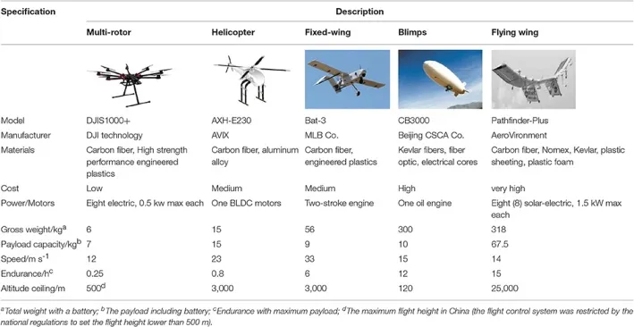
Drones, also known as unmanned aerial vehicles (UAVs), come in various types (Figure 2) and are categorized based on design, purpose, and capabilities. Fixed-wing drones resemble traditional airplanes with a rigid wing structure and are used for long-range mapping, surveillance, and agricultural monitoring. They offer longer flight times, greater speed, and better fuel efficiency. They will be the subject of the article.
Rotary-wing drones include multirotor drones (like quadcopters) and single-rotor helicopters. They are popular for aerial photography, inspections, and short-range transport due to their vertical takeoff and landing, hovering capabilities, and maneuverability. However, they generally have shorter flight times compared to fixed-wing drones.
2 Method Overview
Numerical simulation is crucial for the aerospace industry. Still, it can be slow and expensive in a product design context due to the necessity of rerunning simulations in an iterative design process. The NC Neural Concept platform solves this issue by using Geometric Convolutional Neural Networks to create surrogate models of simulations that run almost in real-time. These surrogate models can manage different shape parameters and utilize data from multiple sources, making the design process more efficient than traditional methods like Gaussian Process regressors.
2.1 Numerical Optimization with Neural Concept
In recent decades, numerical simulation has become crucial for the industry. However, the need to rerun a simulation every time an engineer wants to modify the designed shape slows the engineering process and makes it costly.
The typical approach involves testing only a few designs without searching for potential variations. This limitation has prompted numerous attempts to automate the shape optimization process, but none have succeeded. A classical approach to reducing computational complexity is to use surrogate modeling via Gaussian Process regressors or others, trained to interpolate the performance landscape given a low-dimensional parametrization of the shape space. This interpolator is then used as a proxy for the true objective to speed up the computation, referred to as Kriging in the literature.
However, those regressors are only effective for shape deformations that can be parameterized using relatively few parameters, and their performance hinges on a well-designed parameterization. Furthermore, the regressors are specific to a particular parameterization, and pre-existing computed simulation data using different ones cannot be easily leveraged.
The NC platform uses 3D Deep Learning to create surrogate models of numerical solvers, such as CFD for drone aerodynamics. Shape parameters do not limit NC. NC can be trained with large amounts of data for multiple optimization tasks. Unlike Kriging methods, NC does not require engineers to adhere to a specific parametrization throughout the process; thus, it can combine simulations from various sources and parameterizations using its transfer learning capabilities.
NC is the only CAE-oriented Deep Learning code that can directly work on raw unstructured 3D data without preprocessing it. It leverages multi-scale geometric neural networks by combining surfaces, such as geodesic and Euclidean network architectures.
NC can learn to emulate simulators and reproduce multiple outputs, such as integrated scalar values, e.g., drag forces, energy consumption, or surface and volumetric field values.
2.2 Numerical Simulation with AirShaper
AirShaper is a cloud-based HPC (high-performance computing) platform for external aerodynamics. It automates the entire aerodynamics simulation process from a 3D model to a finished CFD (computational fluid dynamics) simulation.
The required input is limited to the 3D file, the model scale, position, and orientation. The output includes a report with data (including drag and lift values) and aerodynamics visualizations, an online 3D viewer, and the full flow field data in the CFD OpenFOAM format. The platform offers steady-state RANS (Reynolds-Averaged Navier Stokes) simulations using the k-ω SST turbulence model. It is directly compatible with non-watertight 3D CAD models, eliminating the need for CAD repair tedious efforts.
An Application Programming Interface (API) is also available to initiate and process simulations on AirShaper within another software application. AirShaper was awarded ”Motorsport Technology of the Year 2019” for its merits in the automotive segment.
2.3 Optimization Approach
The project aims to optimize the drone aerodynamics performance of one of SenseFly’s increasingly popular drones while still satisfying aerodynamic and geometric constraints.
Engineers working on this case had access to three levels of aerodynamics simulation fidelity.
The first level of fidelity gives an approximate estimate of the aerodynamics simulation results and corresponds to simulations generated by an internally set simulator.
The second simulation fidelity level is the concept aerodynamics simulation from AirShaper, while the third simulation is the most accurate and corresponds to a detailed simulation from AirShaper.
The simulation's detailed (high) fidelity level is quite expensive. Indeed, we only had a budget of 50 such simulations. Fifty cases are too small to optimize a design efficiently in a high-dimensional design space like the one at hand.
With the optimization framework within NC, we pre-trained a geometric neural network with lower-accuracy simulations. Later, the neural network was fine-tuned with higher accuracy simulations to perform the final optimization at the highest level of fidelity, as summarized in Figure (3).

Denoting by Ω the set of feasible geometries, the problem reads as follows:
minimize [-L(V) / D(V)] for V ∈ Ω ⊂ ℝᴺˣ³ subject to Mᵧ (V) = 0
We used NC's optimizer to set up an optimization loop between the neural network and the simulation software. The simulation software is called back automatically to generate new simulation samples, which are then used to retrain the neural network using a specific internal strategy.
3 Setup in NC
We will show how the NC framework optimizes drone design by parametrizing vertex deformation. The primary objective is maximizing the drone's lift-to-drag ratio while ensuring a minimum lift value, using pre-trained neural networks for optimization.
3.1 Optimization in NC
To reduce the number of optimization variables, ensure a smooth surface deformation, and handle the geometric constraints, a parametrization of the vertices V=P(V⁽⁰⁾,z) is introduced where V⁽⁰⁾ denotes the original vertices and z is a vector of the new design variables.
The NC framework lets the user define a set of parametrization modules that can be stacked to generate and optimize deformations relative to an initial design.
All the modules can be interchanged at any point in the optimization process. The shape constraints representing the electronics case that needs to be fitted inside the shape can also be defined as a ”projection” parameterizer.
As described in Figure (4), within the NC framework, we can define all these components separately and connect them to perform the optimization, particularly to propagate the derivatives for gradient-based optimization. NC lets the user define the objective, the neural network, and the parametrization module independently and connects them within the optimization framework.

3.2 Parametrization
We define P⁽ⁱ⁾(z⁽ⁱ⁾,V) as a continuous and differentiable transformation of the input vertices V, from SenseFly’s initial design, according to a variables vector z⁽ⁱ⁾. Moreover, we indicate as P⁽ⁱ⁾◦P⁽ʲ⁾ the composition of two parametrizations.
We now report the three types of parametrization that we used:
- Radial Basis Function (=RBF) interpolation
- Projection Pₚᵣₒⱼ
- Rotation θ
3.2.1 Radial Basis Functions
To smoothly deform the surface, we rely on the RBF deformation of the shape. In this work, we use 50 control points chosen on the surface using farthest point sampling heuristics. Every point can move in all three spatial directions, so we have 150 RBF optimization parameters.
In Figure 5 (a), we show the reference geometry (blue) and a random configuration where the 50 control points C (red) are randomly deformed with |Di,j| ≤ 0.02. The image shows a reference geometry (blue) and a random configuration with control points C (red) and deformed control points C + D (light blue).

Figure 5 (b) shows the projection accomplished by the parametrization Pₚᵣₒⱼ on the fuselage box.

3.2.2 Projection
This parametrization ensures the geometric constraints are satisfied at each iteration of the optimization process.
The fuselage must be at least a rectangular cuboid with dimensions l = 220 X 75 X 30 [mm] (see Figure 6): a vertex must be projected back on its surface before it enters the fuselage volume. The deformed vertices on the rectangular cuboid are projected through a linear map.
Defining as y the deformed position of a vertex and as x its original position, the following must hold:
yᵢ + (xᵢ-yᵢ) tᵢ = sign(xᵢ) lᵢ, for i = 1,2,3.
Among the three candidates (i=1,2,3), the one satisfying the following equation is selected:
-l ≤ y+ (x-y) tᵢ ≤ +l
We will denote this projection operation as Pₚᵣₒⱼ(V).
Figure (6) shows the geometric constraints. The objective block lets the user define an objective function to optimize. The framework automatically stores and logs the objective values of the surrogate model and the ground truth.

3.2.3 Rotation
Given an axis s, specified by two points p₁ and p₂, and a rotation angle θ, the rotation of x₀ around s is given as an additional parameter. This parametrization is used to vary the angle of attack θ of the drone (a rotation around the y-axis); however, it could also be used to rotate some specific parts of the geometry, such as the elevators. It adds one optimization parameter that corresponds to the rotation angle. Since the projector parametrization is stacked before the rotation, the constraint box ”rotates” with the angle of attack.
3.3 Geometric Neural Network
As a Geometric Neural Network regressor, we use the ”PointRegressor” defined by the NC framework Figure 7 illustrates the architecture of our neural network.
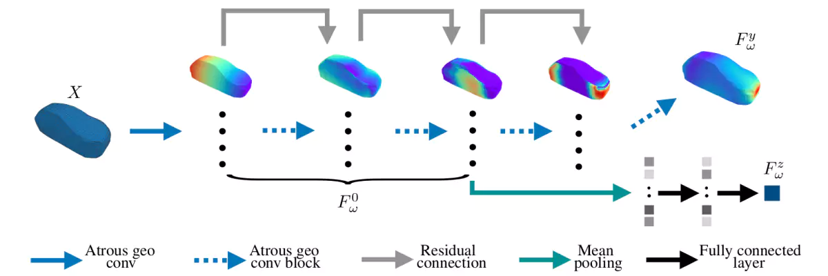
The first part of the model preprocesses the input and constructs a set of features using the previously introduced geodesic convolution operations. These operations predict the global scalars via average pooling and two dense layers. The second branch of the neural network generates pressure fields, relying on an additional set of geodesic convolutions and point-wise operations.
The new neural network takes advantage of a GPU-efficient implementation of geodesic convolutions, eliminating the need for Cube-Mesh mapping or any other prior re-meshing.
3.4 Objectives
The goal was to maximize the drone's lift-to-drag ratio while guaranteeing a minimum lift value. Neural Concept offers a module to define an optimization objective and constraints as a function of the neural network prediction's output.
The objective is maximizing the L/D ratio while constraining lift above L = 8.0 [N].
4 Results
As a first step, we run a full optimization against low-fidelity aerodynamics simulations.
In the second phase of the optimization, we aim to reuse the pre-trained neural network from §4 to initialize the surrogate model.
4.1 Pre-Training Optimization
We first ran a full optimization against low-fidelity aerodynamics simulations. This first aerodynamics optimization is used to start focusing the optimization on potentially interesting designs and to pre-train the neural network.
Figure 8 shows how the objective (the lift-to-drag ratio L/D) evolves over the optimization process iterations. The ground truth and neural network predictions are shown with their centered moving average (with a window size of n = 20). Moreover, the relative error (and its moving average) are also shown.

The figure also shows that the mean objective value increases over time. The reference objective represents the maximum value of the lift-to-drag ratio obtained by simulating the reference geometry for Nθ = 20 equispaced angles of attack −2° ≤ θ ≤ 7°. Even though the moving average is smaller than the reference objective, our interest is to find an increasing number of geometries that are better than the eBee.
4.2 Transfer Learning
In the second phase of the optimization, we reuse the pre-trained neural network from §4 to initialize the surrogate model. The initial surrogate model will optimize the design against the ”accurate” simulation from AirShaper.
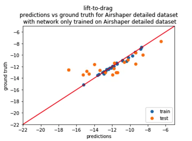
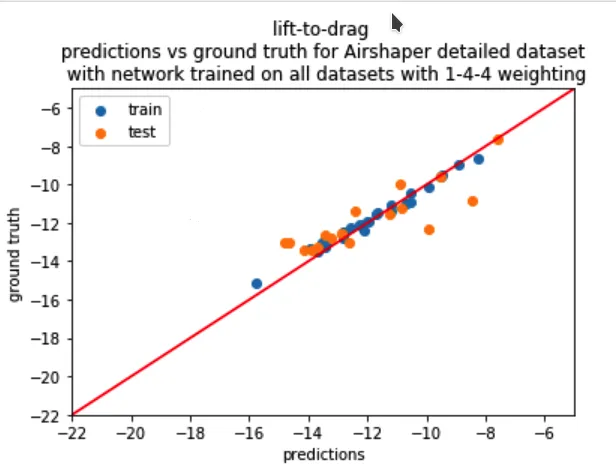
Figure 9 shows the advantage of using a pre-trained neural network to initialize the second optimization phase in terms of a KPI known as the coefficient of determination R².
Figure 9(a) shows the model's performance when trained directly with 50 high-fidelity simulations, yielding R² = 30.4%.
In Figure 9(b), the model was pre-trained before using low-fidelity simulations. Pre-training with all datasets yields a superior value of R² =54.2% and therefore brings more than 20% improvement in R², which motivates the transfer-learning approach.
4.3 Final Design
By comparing the original design to the optimized one, the lift-to-drag ratio has increased by 4.25%, and the drag has been reduced by 6.25% at maximum L/D starting from the initial geometry shown in Figure 10. The optimization process was run using only 40 detailed simulations and can converge to much more efficient designs.
It is interesting to see that the automatic optimization algorithm converges to some shapes and techniques that have been applied before in aviation.
The result in Figure 11 is a more "organic" shape, featuring:
- Anhedral wing setup: the wings of the optimized design feature a more pronounced anhedral setup (wings pointing downward). This will influence the pressure pattern on the wings and, although not included in the goal of this optimization, will also result in a more dynamic response of the drone (as opposed to the self-stabilizing effect of a dihedral wing setup wings pointing upward).
- Variable angle of attack: the angle of attack of the airfoil section of the wing changes across the length of the wings. In this case, the angle of attack increases towards the root of the wing, where there is interference with the flow around the fuselage.


4.3.1 Winglet Orientation
As shown in Figure 12 (baseline) and Figure 13, the optimized design tilts the winglets inward at the end of the wings to reduce the wingtip vortex.


4.3.2 Fuselage Design
The optimized fuselage features a more airfoil-like design, with a low leading edge and quite a lot of camber along the length (curvature of the main body).
This helps to accelerate the air flows at the top of the fuselage, creating a low-pressure zone that generates additional lift force on the drone body.
Figure 14 shows the drone pressure field. The fuselage of the original design has only a slight camber.

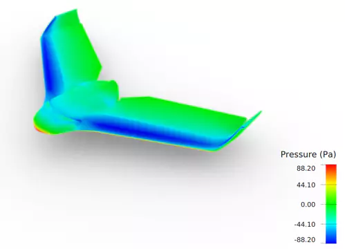
Figure 15 shows the pressure field on the drone. The optimized design has a larger camber on the fuselage, generating additional lift force.


Acknowledgments
We thank the authors and persons who contributed to this report:
- Neural Concept: Juliette Marrie, Pierre Baqué
- AirShaper: Wouter Remmerie
- EPFL: Francesco Bardi, Prof. Pascal Fua

