Response Surface Methodology - Overview & Applications
Response Surface Methodology (RSM) is a collection of mathematical and statistical techniques for modeling and optimizing systems influenced by multiple variables. It focuses on designing experiments, fitting mathematical models to data, and identifying the optimum location for operational conditions.
Key tools include statistical analysis, central composite designs, and other structured experiment plans.
In essence, response surface methods are used to:
- Quantify how input variables jointly affect a response
- Determine optimal variable settings
- Assess the sensitivity of the response to input changes
Here’s an overview of the article contents:
- What Is Response Surface Methodology?
- Why is the History of RSM Important?
- What are the Applications of Response Surface Methodology?
- Designing Response Surface Experiments
- Why Plan an RSM Experiment?
- What is Factorial Design?
- What is Box-Behnken Design (BBD)?
- Other RSM Designs
- Mathematical Modeling & Data Analysis
- Fitting Response Surface Models
- The Quadratic Model
- Regression Analysis in RSM Regression Link to Quadratic Models
- Interpreting Model Coefficients in Quadratic Models
- Data Analysis and Model Fitting in Response Surface Methodology
- Collecting Experimental Data
- Model Fitting and Analysis
- Model Validation and Selection in Response Surface Methodology
- Optimization Using Response Surface Methodology
- Identifying Optimal Process Conditions
- Practical Considerations in Optimization
- Steepest Ascent/Descent Methods
- Desirability Function Approach
- Visualization & Interpretation in RSM
- Contour Plots
- 3D Surface Plots
- Overlaid Contour Plots for Multiple Responses
- Operating Window Identification
- Advanced Modeling Approaches
- Combining Response Surface Modeling and ROM
- Robust RSM Approaches
- Mixture Experiments
- Emerging Trends
What Is Response Surface Methodology?
Response Surface Methodology (RSM) is a collection of mathematical and statistical techniques, often referred to as response surface methodology rsm, used to model relationships between multiple independent variables and one or more responses. It is applied in product and process design to identify optimal conditions and to study how factors interact. RSM belongs to the broader framework of Design of Experiments (DOE), with a specific focus on building predictive models and guiding optimization.
Key aspects of RSM are:
| Key Aspect | Details | Practical Notes / Examples |
|---|---|---|
| Fundamental Concepts and Principles | RSM relies on structured experimental designs such as factorial, CCD, and BBD. It uses polynomial models, usually quadratic, to approximate the response surface and evaluate factor interactions and curvature. | Enables identification of linear, interaction, and quadratic effects. For example, in chemical reactions, temperature and pressure interactions can be quantified to optimize yield. |
| Advantages Over Traditional Approaches | Efficiently explores the design space with fewer runs compared to exhaustive trial and error methods. Directly supports optimization and sensitivity analysis and provides a clear interpretation of factor effects and interactions. | Reduces experimental cost and time. For instance, in material processing, RSM enables identification of optimal heat treatment parameters without testing every possible combination of parameters. |
| Applications Across Industries | Applied in fields like engineering, manufacturing, pharmaceuticals, biotechnology, product design, and quality improvement, where multiple factors influence a response and optimization is needed. | Examples include optimizing engine performance in automotive, tuning fermentation conditions in biotech, or improving tablet formulation in pharmaceuticals. Similar trends are detailed in innovations in aerospace product design, which explores AI plus statistical methods in aerospace component design and aerodynamics. |
Why is the History of RSM Important?
The history of RSM is significant because it demonstrates how the method originated from practical industrial needs and evolved into a formal statistical discipline. Early work by Box and Wilson in the 1950s linked experimental design with optimization, creating tools that could guide process improvement in chemical engineering and manufacturing.
Here’s the historical progression of RSM:
| Period | Key Developments | Impact / Notes |
|---|---|---|
| 1950s | George E. P. Box and K. B. Wilson introduced response surfaces and published “On the Experimental Attainment of Optimum Conditions” (1951). | Established the foundation for RSM, emphasizing systematic modeling of relationships between multiple variables and responses. |
| 1960s–1970s | Industrial adoption of RSM for experimentation. | RSM became an indispensable tool for optimizing processes in manufacturing and chemical engineering. |
| 1987 | Publication of Box and Draper’s “Empirical Model-Building and Response Surfaces.” | Provided a comprehensive guide to RSM, enabling broader adoption across engineering, chemistry, and manufacturing industries; emphasized efficiency and structured experimentation. |
| Recent Years | Integration with computational methods, AI, and machine learning. | Expanded RSM’s capability to model complex, nonlinear systems; modern software tools allow more efficient implementation and optimization in diverse fields. |
What are the Applications of Response Surface Methodology?
Response Surface Methodology is widely applied in industries that require systematic process optimization and optimization of products.
It is used to fine-tune design parameters, improve quality, and reduce experimental costs by extracting maximum information from limited data.
The automotive industry utilizes RSM to optimize combustion for improved fuel efficiency and reduced emissions, calibrate suspension and aerodynamics, enhance material processing such as welding, and support crashworthiness studies through efficient experiments. RSM, a mature statistical tool, complements emerging AI and generative design methods. While AI explores broad design spaces and suggests unconventional solutions, RSM provides rigorous model-based optimization, making it an essential engineering tool for decision-making.
The automotive industry is a competitive arena where new methodologies, such as AI and generative design, are tested, and statistical analysis is well-established in design and manufacturing departments.
Efficiency in Parameter Optimization
In engineering, particularly in the automotive sector, RSM is crucial for optimizing multiple parameters to achieve multiple response optimization. For instance, in automotive design, RSM can optimize fuel efficiency by considering independent variables such as engine compression ratio, fuel injection timing, and air-fuel mixture.
Accelerated Product Development
RSM can accelerate product development processes within the automotive industry, especially through multiple response optimization.
Engineers can iterate on designs more quickly by reducing the need for physical prototypes through virtual experimentation, thereby facilitating numerical optimization.
For example, RSM could streamline the development of a vehicle’s suspension system by optimizing factors like spring rates and damping coefficients.
Robustness in Design
In the competitive automotive landscape, robust design is essential. RSM contributes to ensuring that designs are not only optimized but also robust across various operating conditions. For instance, it can aid in designing a robust braking system by considering factors such as brake pad material, disc diameter, and temperature variations.
Cost Reduction Through Optimization
RSM assists engineers in finding a balance between performance and cost. Optimizing factors such as material usage and manufacturing, automotive engineers can design cost-effective yet high-performance components. An example is optimizing composite materials in automotive body panels to strike a balance between strength, weight, and cost.
Real-World Testing Reduction with RSM
Physical testing is resource-intensive in automotive product development. Cost reduction is possible thanks to the benefits of generative design. RSM helps reduce reliance on extensive real-world testing by accurately predicting how changes in design variables will impact performance. This is exemplified in aerodynamics, where RSM can optimize vehicle shapes for reduced drag without requiring numerous wind tunnel tests.
Environmental Impact Mitigation with RSM
Environmental considerations are integral to automotive design.
RSM aids in optimizing designs for reduced environmental impact, including qualitative factors like enhancing fuel efficiency, reducing emissions, and optimizing electric vehicle battery performance, while considering dependent variables.
In summary, RSM is a valuable tool for engineering and product design in the automotive industry, especially when dealing with several factors . Its technical applications optimize processes, accelerate development, ensure robust design, offer cost-effective solutions, reduce reliance on real-world testing, and promote environmentally conscious design.
Experimental Design in RSM
In Response Surface Methodology, the experimental design specifies how data are collected within the experimental region, which is the domain of interest where factor levels are varied.
The goal is to efficiently explore this area and identify relationships between factors (like temperature, pressure, and concentration) and the response. CCD and Box–Behnken Designs are popular because they provide balanced experimental coverage while minimizing runs. They enable fitting polynomial models that capture main effects, interactions, and curvature, which are crucial for optimization.
Designing Response Surface Experiments
Designing experiments in RSM requires careful planning to ensure systematic and comprehensive coverage of the experimental region, which involves selecting quantitative factors, defining their levels, and choosing an appropriate experimental design to efficiently capture the effects and interactions of these factors.
Factorial designs, including full and fractional factorials, coding strategies, and resolution considerations, serve as the foundation.
They enable the initial screening of factors, identification of significant variables, and guidance for subsequent response surface designs, such as central composite or Box–Behnken designs. Proper planning ensures that the resulting data can support accurate modeling and reliable optimization.
Below find a summary guideline for Designing Response Surface Experiments:
| Step | Purpose | Key Considerations | Example/Notes |
|---|---|---|---|
| 1. Select quantitative factors | Identify input variables affecting the response. | Temperature, pressure, concentration, speed, etc. | Focus on controllable and measurable variables. |
| 2. Define factor levels | Determine the range and granularity of each factor. | Minimum, maximum, center points. | Ensures the experimental region is well covered. |
| 3. Choose a factorial design | Screen factors and detect main effects and interactions. | Full or fractional factorial, coding, resolution. | Fractional factorial reduces runs while preserving key information. |
| 4. Apply RSM design | Model response surface and capture curvature. | Central Composite Design, BBD. | Builds on initial factorial results for optimization. |
| 5. Collect and analyze data | Fit polynomial models and evaluate interactions. | Check model adequacy, residuals, and significance. | Supports optimization and sensitivity analysis. |
Why Plan an RSM Experiment?
Planning an RSM experiment is a crucial first step that requires careful attention. The goal is to systematically explore how factor settings affect the measured response variable. Before implementing RSM, researchers must clearly define project objectives and the study’s scope to ensure the design aligns with intended outcomes.
The key components in planning include:
- Identification of Factors: Clearly define the factors that may influence the response. These input variables could be process parameters, material properties, or other relevant variables.
- Selection of Factor Levels: Determine the range and levels at which each factor will be tested for a comprehensive understanding of the factor space.
- Experimental Design: Choose an appropriate experiment design that optimally utilizes resources while providing robust information. Standard designs include factorial experiments, CCD, and BBD.
What is Factorial Design?
Central Composite Designs are a key tool in RSM for modeling curvature and building second-order polynomial models. CCDs extend factorial designs by adding center points and axial (star) points, allowing estimation of both linear and quadratic effects.
Key Components of Factorial Design
- Factorial points: Represent all combinations of factor levels (as in a standard factorial design).
- Center points: Repeated runs at the midpoint of the experimental region to estimate experimental error and check model adequacy.
- Axial (star) points: Axial (star) points extend beyond the factorial points to capture curvature in the response surface. Positioned along each factor axis at a distance α from the center, they allow estimation of quadratic effects for each factor individually. Star points represent the extremes of the experimental region along each axis, providing critical information about how the response behaves at higher and lower factor levels.
- Rotatability: CCDs can be arranged to be rotatable, meaning the variance of predicted responses is constant at points equidistant from the center, ensuring uniform precision across the region.
Variations of Factorial Design
- Circumscribed CCD: Axial points lie outside the factorial cube.
- Inscribed CCD: Factorial points are scaled to fit within the axial range.
- Face-centered CCD: Axial points lie on the faces of the factorial cube, simplifying experimentation but reducing rotatability.
CCDs allow for the estimation of main, interaction, and quadratic effects, and support reliable optimization in RSM, which can be visualized using a contour plot.
What is Box-Behnken Design (BBD)?
BBD is a choice when a full factorial experiment is impractical due to resource constraints. It efficiently explores the factor space with fewer experimental runs than a full factorial design. The formula for the number of runs in a BBD is given by:
Number of runs = 2k × (k – 1) + nₚ
where k is the number of factors, and nₚ is the number of center points.
BBD is beneficial for exploring quadratic response surfaces.
- BBD Example
For a Box–Behnken Design (BBD) with three factors (k = 3) and one center point nₚ=1 in the formula for BBD runs 2k × (k – 1) + nₚ, we get:
2 × 3 × (3 – 1) + 1 = 2 × 3 × 2 + 1 = 12 + 1 = 13 runs
Here is a table showing all 13 runs for a 3-factor Box–Behnken Design with one center point (we assumed the factors to be A, B, and C, each at two coded levels: -1 (low) and +1 (high)).
| Run | A | B | C |
|---|---|---|---|
| 1 | -1 | -1 | 0 |
| 2 | -1 | +1 | 0 |
| 3 | +1 | -1 | 0 |
| 4 | +1 | +1 | 0 |
| 5 | -1 | 0 | -1 |
| 6 | -1 | 0 | +1 |
| 7 | +1 | 0 | -1 |
| 8 | +1 | 0 | +1 |
| 9 | 0 | -1 | -1 |
| 10 | 0 | -1 | +1 |
| 11 | 0 | +1 | -1 |
| 12 | 0 | +1 | +1 |
| 13 | 0 | 0 | 0 |
| Notes | |||
| “0” indicates the center level of the factor. Each factor combination explores the midpoints of edges of the cube (Box Behnken structure). The center point allows estimation of pure error and checks model adequacy. | |||
Other RSM Designs
Beyond Central Composite Designs, several alternative RSM designs are used depending on experimental constraints, factor types, and optimization goals.
These designs complement classical CCD and Box–Behnken methods, providing flexibility for complex regions, high-dimensional spaces, or constraints. They enable efficient data collection and reliable modeling for RSM optimization.
| Design | Key Features | Typical Use Case |
|---|---|---|
| Doehlert Design | Factors arranged in a hexagonal pattern allow uniform precision with fewer runs. | When a small number of experiments is needed and uniform coverage of the experimental region is desired. |
| Uniform Shell Design | Factorial points placed on the surface of a hypersphere; highly uniform distribution. | Optimization in high-dimensional factor spaces where rotatability is important. |
| D-Optimal Design | Uses algorithmic selection of points to maximize statistical efficiency (determinant of information matrix). | For irregular experimental regions or when some factor combinations are infeasible. |
| Mixed-Level Design | Factors can have different numbers of levels. | When some variables are categorical or require finer resolution than others. |
| Constrained Design | Factor levels restricted due to practical limitations. | For experiments with physical, safety, or cost constraints. |
Mathematical Modeling & Data Analysis
Fitting Response Surface Models
Once data are collected from your RSM experiment, the next step is to fit a mathematical model that describes how your variables interact.
The Quadratic Model:
- Suppose the dependent variable is Y, and the independent variables are Xᵢ and Xⱼ.
- The aim is to represent Y as a function of these inputs: Y = Y(Xᵢ, Xⱼ).
- A standard quadratic RSM is expressed as: Y = β₀ + ∑ᵢ βᵢ Xᵢ + ∑ᵢ ∑ⱼ βᵢⱼ Xᵢ Xⱼ + ε
- where the symbols are explained in the table below.
| Term | Description | Explanation |
|---|---|---|
| β0 | Intercept | The value of Y when all Xi are zero. |
| βi | Linear coefficients | Show how Y changes with a unit change in a single Xi. |
| βij | Interaction coefficients | Capture how pairs of variables (Xi and Xj) jointly affect Y. |
| Xi, Xj | Independent variables | The factors we control or vary in the experiment. |
| ε | Error term | Accounts for variation not explained by the model. |
- Regression Analysis in RSM
- Fitting the model uses regression analysis, typically via least squares, to estimate coefficients (β₀, βᵢ, βᵢⱼ). Transformations may improve linearity or stabilize variance. Multicollinearity (highly correlated factors) can affect estimates and interpretation, so designs and coding strategies are chosen to minimize it.
- Regression Link to Quadratic Models
- Regression is the method that turns data into the quadratic model described above. Without regression, the coefficients and interactions remain unknown, and the response surface cannot be quantified or used for optimization. Essentially, regression bridges the raw experimental observations and the empirical model, allowing for accurate predictions.
Interpreting Model Coefficients
Interpreting the coefficients within the response surface model is pivotal for discerning the quantitative impact of each variable on the predicted response amount.
The coefficients βᵢ (linear coefficients) and βᵢⱼ (interaction coefficients) translate the strength and direction of the relationships:
- The strength of a coefficient βᵢ tells us how much Y changes when the corresponding independent variable changes by one unit. Think of it as the power of influence each variable wields.
- The direction βᵢⱼ is where it “gets exciting”.
- A positive coefficient implies a positive influence on Y. Example: Picture it as your variable being a cheerleader, lifting the Y higher.
- Conversely, a negative coefficient suggests a negative impact. Example: imagine a subtle force pulling the Y in the opposite direction.
Examples of βᵢ and βᵢⱼ in a Quadratic Model:
| Coefficient | Example Variable(s) | Example Value | Interpretation |
|---|---|---|---|
| Linear coefficient β1 | Temperature (X1) | β1 = 2 | For each +1 unit in temperature, Y (product yield) increases by 2 units. |
| Linear coefficient β1 | Temperature (X1) | β1 = -1 | For each +1 unit in temperature, Y decreases by 1 unit. |
| Interaction coefficient β12 | Temperature (X1) and Pressure (X2) | β12 = 3 | Increasing both temperature and pressure together enhances Y. |
| Interaction coefficient β12 | Temperature (X1) and Pressure (X2) | β12 = -2 | Increasing temperature and pressure together dampen Y. |
Data Analysis and Model Fitting in Response Surface Methodology
Data analysis and model fitting are crucial for extracting actionable insights from RSM experiments, including validating models, estimating effects, testing for significance, and interpreting coefficients to understand the relationships between variables.
Collecting Experimental Data
Data acquisition in RSM involves executing planned experimental runs and measuring responses to capture the effects and interactions of factors accurately within the experimental domain. For example, when optimizing a chemical reaction, factors such as temperature, pressure, and concentration are varied systematically, and responses, including yield, reaction time, and purity, are recorded to ensure the dataset reflects the system and supports reliable modeling.
Model Fitting and Analysis
Once the data are collected, models are fitted through regression analysis. Effect estimation shows how much each factor and interaction influence the response. ANOVA tests the statistical significance of the model, terms, and fit. Coefficients quantify factor impacts, and significance testing confirms effects are unlikely due to chance.
Collectively, these steps enable the RSM experiment to transition from raw observations to a validated response surface model that supports optimization and decision-making.
Model Validation and Selection in Response Surface Methodology
The validation and selection of a response surface model involve scrutinizing its predictive accuracy and generalizability to unseen data.
Techniques such as cross-validation and goodness-of-fit measures help assess the model’s robustness and applicability beyond the observed data.
Optimization Using Response Surface Methodology
In Response Surface Methodology, optimization is the toolset guiding engineers toward efficiency and performance goals. Let’s explore the tools and considerations that make optimization an actionable toolset in the Response Surface Method.
Identifying Optimal Process Conditions
RSM acts as a “treasure map” in our quest for optimal process conditions. By tweaking the factor level, we aim to find the combination that maximizes or minimizes our response variable.
Picture it as exploring a terrain where each adjustment brings you closer to the optimal summit. Through its systematic approach, RSM ensures we reach the highest peaks or navigate the deepest valleys, depending on the process optimization goal.
Practical Considerations in Optimization
When we optimize complex processes using the Response Surface Method, it’s like fine-tuning a machine, a systematic approach to make things work better. As we embark on this optimization journey, with many factors at play, practical considerations become our guiding tools, enabling us to make informed decisions in the face of challenges.
- One vital consideration is ‘addressing constraints,’ which means dealing with system limits like time, budget, or equipment capacity during process optimization. Thus, solutions are practical and feasible, avoiding unrealistic scenarios.
- Another important aspect is ‘ensuring robustness,’ which involves making solutions strong enough to handle unexpected problems. In product design, this means testing in real-world conditions or adjusting for input variations to ensure effectiveness despite uncertainties or environmental changes.
- Last but not least, ‘avoid overfitting.’ Avoiding overfitting is like not getting lost in the details. In optimization, overfitting occurs when a solution is too tailored to specific data, making it less useful elsewhere. To avoid this, focus on essential patterns without unnecessary details, ensuring solutions work in both lab and real-world settings.
Steepest Ascent/Descent Methods
Steepest ascent/descent methods are iterative techniques in RSM used to move toward an optimal response quickly.
Starting from an initial experimental point, the method follows the direction of maximum increase (ascent) or decrease (descent) based on estimated factor effects from a fitted model. Experiments are conducted along this path until the response stops improving, signaling proximity to the optimum.
This approach is efficient for locating the region of interest before applying more detailed designs, such as central composite or Box–Behnken, thereby reducing the number of experiments needed to reach optimal factor settings.
Desirability Function Approach
Think of the desirability function approach as your guide or compass through the optimization journey.
This method doesn’t settle for just one target; it simultaneously plays with multiple response variables and their respective targets. The formula for desirability (D) encapsulates your “aspirations”:
D = (d₁ × d₂ × … × dₖ)^(1/k)
Here, d₁, d₂, …, dₖ are individual desirabilities for each response, and k is the number of responses.
Visualization & Interpretation in RSM
Visualization is a crucial step in RSM, enabling the interpretation of models and communicating how factors impact responses.
Standard visualization tools include:
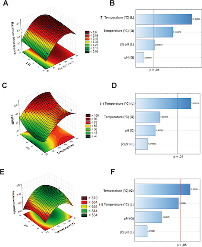
- Contour Plots
- 2D representations showing lines of constant response. They highlight regions where the response meets specific criteria and help identify trends and interactions between two factors.
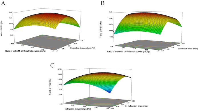
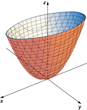
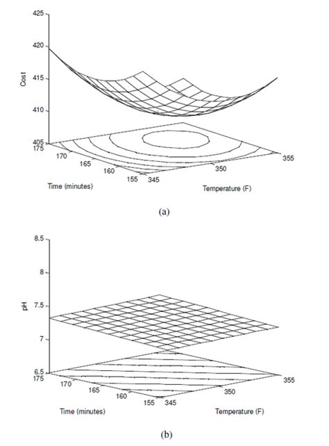
- 3D Surface Plots
- Three-dimensional plots of the response surface. These provide an intuitive view of curvature, interactions, and optimal regions across the experimental space.
- Overlaid Contour Plots for Multiple Responses
- Used when optimizing multiple responses simultaneously. Overlaid contours allow identification of regions that satisfy multiple criteria, facilitating multi-objective decision-making. A useful comparison of optimization vs generative design helps clarify how RSM’s structured experimentation differs from generative design’s broader, often less constrained search of design space.
- Operating Window Identification
- Visualization helps define the range of factor levels (the operating window) where the process meets the desired performance and quality targets, guiding robust process design and practical implementation.

Advanced Modeling Approaches
Beyond traditional polynomial models, advanced methods extend RSM’s capabilities. Techniques include:
- Kriging
- Provides spatial interpolation and captures nonlinearity.
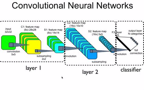
- Neural Networks
- Model highly nonlinear responses with flexibility.
- Fuzzy Logic
- Handles uncertainty and imprecision in factor effects.
- Bayesian Methods
- Incorporate prior knowledge and quantify uncertainty.
- Multi-Response Models
- Optimize several outcomes simultaneously.
Combining Response Surface Modeling and ROM
Balancing accuracy and efficiency is a constant challenge. Combining RSM with Reduced Order Modeling (ROM) allows the construction of cost-effective surrogates for complex systems. This aligns with ideas explored in simulation-driven design, where surrogate models are used together with simulations to speed up product development.
- Step 1: RSM Insight – Initial experiments identify key variables and interactions, providing a cost-effective understanding of system behavior.
- Step 2: ROM Development – ROM captures essential dynamics using a reduced set of basis functions or modes, significantly cutting computational cost.
In automotive battery optimization, for instance, RSM identifies key parameters like charge-discharge rates, temperature, and electrode composition. ROM then creates a surrogate model based on these, enabling rapid simulations and iterative optimization. The ROM approach speeds up design refinement while maintaining accuracy.
Robust RSM Approaches
Robust RSM accounts for variability and uncertainty in real-world systems, often using an extreme vertices design. Techniques include:
- Noise factor analysis to evaluate process sensitivity
- Tolerance design to ensure consistent performance
- Uncertainty quantification to inform decision-making under variability
Mixture Experiments
Mixture experiments study systems where the proportions of components influence the response. A key characteristic of mixture designs is that factor proportions must sum to a fixed total (e.g., 100%), which makes them different from standard factorial designs.
Common designs include:
- Simplex-Lattice: ensures uniform coverage of the mixture space.
- Extreme Vertices: focuses on boundary regions of feasible mixtures.
- Constrained Mixtures: respects practical or physical limits on component proportions.
- Mixture-Process Combinations: integrates mixture ratios with process variables to study their combined effect.
Emerging Trends
RSM continues to evolve, integrating with new technologies and methodologies:
- Machine Learning Integration
- Enhances predictive capability for complex responses
- Big Data
- Supports high-dimensional experimentation and real-time feedback
- Adaptive RSM
- Dynamically updates designs based on ongoing results
- Sustainable Optimization
- Incorporates environmental and resource constraints into experimental planning
FAQs
How Does Response Surface Methodology Compare with Other Optimization Techniques?
RSM is model-based and statistically rigorous, offering insight into factor interactions within the defined experimental domain. Compared to trial-and-error or gradient-free methods, it requires fewer experiments and provides interpretable polynomial models, but it may not scale efficiently to very high-dimensional spaces.
What are the Main Steps Involved in a Response Surface Methodology Experiment?
Steps include selecting quantitative factors, defining factor levels, choosing a factorial or response surface design, conducting experiments, collecting data, fitting a polynomial model, performing regression and ANOVA, and identifying optimal conditions.
What are the Limitations of Response Surface Methodology?
RSM assumes smooth, continuous responses and may fail for highly nonlinear or discontinuous systems. It can be inefficient for very high-dimensional problems and sensitive to measurement noise or multicollinearity among factors.
Can You Provide Examples of Response Surface Methodology in Real-World Applications?
Examples include optimizing chemical reaction yields, adjusting fermentation parameters in biotechnology, tuning polymerization conditions, enhancing automotive engine efficiency, and calibrating manufacturing processes in the electronics industry.
How is Response Surface Methodology Used in Optimization Processes?
RSM models the relationship between input factors and response variables, then identifies settings that maximize or minimize the target variable. Contour plots, 3D surfaces, and multi-response overlays guide the selection of optimal conditions.
What are the Advantages and Disadvantages of Response Surface Methodology?
Advantages: systematic, interpretable, efficient, captures interactions and curvature. Disadvantages: limited to very high-dimensional or highly nonlinear systems, sensitive to experimental error, requires careful design to avoid multicollinearity.
How does Multi-Response Optimization use Desirability Functions to Handle Multiple Variables?
In multi-response optimization, desirability functions combine the effects of several variables in a dimensional space, accounting for linear terms and interactions to identify the best compromise solution.
What are the Main Applications of Response Surface Methodology in Chemical Engineering?
RSM is used to optimize reaction conditions, improve yield, study factor interactions, and design robust processes. Typical applications include chemical synthesis, catalyst optimization, separation processes, and formulation development.
Bibliography
- Box, G. E. P., & Wilson, K. B. (1951). On the Experimental Attainment of Optimum Conditions. Journal of the Royal Statistical Society: Series B (Methodological), 13(1), 1-45.
- Box, G. E. P., & Draper, N. R. (1987). Empirical Model-Building and Response Surfaces, John Wiley & Sons.
- Myers, R. H., Montgomery, D. C., & Anderson-Cook, C. M. (2016). Response Surface Methodology: Process and Product Optimization Using Designed Experiments (4th ed.). John Wiley & Sons.
- Khuri, A. I., & Cornell, J. A. (1996). Response Surfaces: Designs and Analyses. Marcel Dekker.
- Draper, N. R., & Box, G. E. P. (2007). Response Surface Designs: A Literature Survey. Technometrics, 49(2), 121-135.