What Is Dynamic Simulation? Engineering Applications & Methods

This article explores a technology that models how systems change over time. Unlike static simulations (assuming no motion) and steady-state simulations (representing stable conditions where variables no longer change), dynamic simulation captures evolving behaviors.

Dynamic simulation provides a higher level of process analysis than static or steady-state simulations. Dynamic models illustrate how mass and energy accumulate and evolve within a system over time. They focus on transients, cycles, and complex interactions, such as the coupled physics between solids and fluids. Dynamic simulation allows engineers to analyze fatigue, resonance, turbulence, and heat dissipation to predict failures and optimize performance before a prototype is built.

3D engineering analyses (CAE) are implemented with FEA software for stress analysis and CFD for fluid mechanics or heat transfer. CAE helps refine designs early, reducing costly trial-and-error and minimizing later operational risks on-site. This is thanks to very realistic digital representations of engineering and other events with better insights into product and process design and many different areas, such as logistics. We will also explore new Machine Learning applications to make those analyses even cheaper and faster.

We will show examples of this technology in product and process design improvement. The digital approach identifies potential issues, tests new designs, and improves system performance on-site.

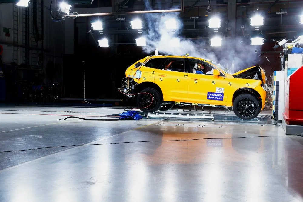
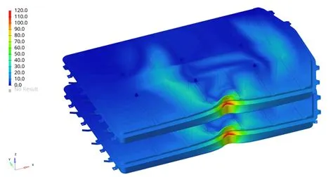
Take automotive crashworthiness as an example. FEA models the vehicle's transient behavior during a collision, helping engineers optimize crumple zones and safety features to minimize injury and improve vehicle design before physical crash tests.

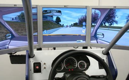
Dynamic simulations model complete driving cycles to evaluate vehicle fuel consumption, accounting for time-varying factors like acceleration, braking, and speed.

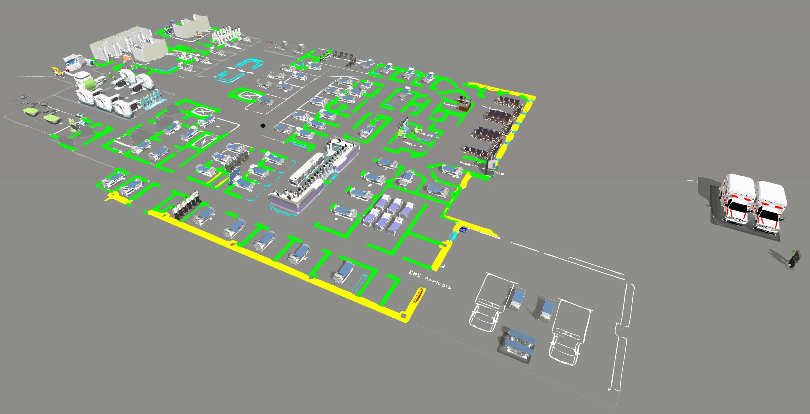
Dynamic models help engineers identify and overcome bottlenecks by simulating how systems evolve.

As another example of the numerical or digital approach, simulation users model the flow of materials through different stages in a manufacturing process to reveal where delays or congestion occur. The identified bottleneck can be a machine or conveyor slowing down an entire distribution process.

Fundamental Principles of Dynamic Simulation

Dynamic simulations are part of the broader field of engineering simulation. They track how systems evolve, using differential equations to model transients, oscillations, or steady states in engineering processes.

Time-Dependent Behavior

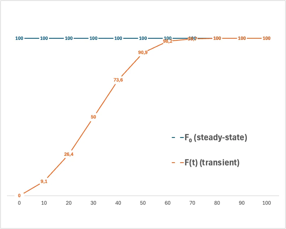
System state variables can evolve due to external or internal factors. The evolution can exhibit transients, oscillatory, or steady-state behaviors. Examples include temperature changes in reactors and pressure variations in hydraulics. The time-dependent behavior can be limited, such as in the case of a physical system with a parameter F(t) reaching a relaxation state F0, as in the figure.

This convergence from transient to steady state can also reverse. A steady-state system may undergo a Hopf bifurcation and begin oscillating. The figure illustrates a supercritical Hopf bifurcation: β controls stability and the nature of fixed points. β<0 means the system spirals inward, β=0 indicates bifurcation, β>0 leads to sustained oscillations in a limit cycle around the unstable fixed point.

‍

In other cases, like in turbulence (figure), the system does not settle into a simple steady state; there is a continuous interplay of vortices, energy cascades, and fluctuating structures across multiple scales. Even if the time-averaged quantities <F> (e.g. mean velocity or pressure) might appear steady, and this is exploited by simulation approaches like CFD-RANSE, the instantaneous flow remains chaotic and highly dynamic due to the fluctuating component F'(t).

Unlike turbulence, which involves chaotic and broadband fluctuations, dynamical systems like the Van der Pol oscillator (figure) have a well-defined periodic behavior. However, they can exhibit chaotic dynamics if driven by strong external forces.

Mathematical Foundation

Dynamic simulation relies on differential equations to describe the evolution of variables. By knowing the rates of change dF/dt, we can reconstruct their values F(t) at any given instant with numerical methods that depend on t (ODEs) or additionally also spatial variables (PDEs).

To define the problem, we need:

• Initial conditions (i.e. starting values F₀) for both ODEs (F₀) and PDEs (F₀(x,y,z));
• Boundary conditions are required for PDEs, i.e., F evaluated at the spatial boundary (F|∂Ω) of the system domain Ω.

Steady State vs. Dynamic Simulation: Key Differences

Steady-state analysis represents a system under conditions where variables do not vary over time. 

Steady-state simulation of constant fluid flow is used for most industrial analyses. In this case, Reynolds-Averaged CFD solves statistically steady flow: no transient effects are resolved. LES (Large-Eddy Simulation) solves instead the inherently unsteady evolution of large turbulence eddies that steady-state simulation cannot capture. LES of hybrids with Reynolds-Averaged become essential for specific situations such as aero acoustics. In most cases, such as modelling a valve opening, unsteady Reynolds-Averaged can reach sufficient accuracy for industry purposes.

Dynamic Simulation Models in Engineering

Now, let us distinguish between the discrete and continuous models. Engineers are more familiar with the latter.

Types of Simulation Models

Discrete Event Simulation represents situations where state evolutions occur at discrete points driven by events. In manufacturing and logistics, it tracks individual entities and resource utilization.

Continuous Simulation represents systems that evolve continuously. These systems are often governed by differential equations, which numerical methods like CFD solve.

Hybrid Simulation combines discrete event and continuous models, handling interactions between event-driven è continuous processes (e.g., hydraulic systems + control logic).

Industry Applications of Continuous Simulation

Continuous dynamic analysis models behaviors in complex industrial scenarios.

In the automotive industry, it helps analyze crashworthiness, aerodynamics, and powertrain performance to improve safety and efficiency.

In aerospace, it is used for turbulence studies, flight envelopes, and propulsion efficiency, ensuring better performance and stability in external aerodynamics.

It optimizes renewable energy integration, HVAC performance, and grid stability in energy systems, enabling better resource management.

Dynamic Simulation in Process Engineering

We will now tackle Process Engineering Simulation in industrial applications.

What is Process Engineering Simulation? Typical Applications

Dynamic process simulation is used to optimize time-variant processes in Chemical Process Control, such as pipelines, mixers, and various types of heat exchangers. 

The aim is to predict responses to changes in operating conditions and implement control strategies. For example, we analyze fluid flow in pipelines, capturing pressure drops, heat transfer, and system phase behavior. This method shows how temperature, pressure, and flow rate variations impact the process.

Batch and semi-batch processes can only be successfully modeled in dynamic simulators. Batch processes capture the startup, reaction, and shutdown phases.

Continuous processes may utilize both steady-state and dynamic approaches depending on operating conditions.

Case Study: Chemical Reactor Process

Steady-state analysis optimizes continuous stirred-tank reactor operations by solving mass and energy balances under constant conditions, ensuring efficient chemical production. However, real-world processes exhibit transient behaviors such as startup, shutdown, and disturbances. Dynamic simulation evaluates stability, control performance, and emergency response. A hybrid approach combines steady-state optimization with dynamic analysis, improving process control and ensuring safe, efficient operations under varying conditions. This enhances reliability and adaptability in industrial chemical processes.

Advantages and Challenges of Dynamic Simulation

Dynamic simulation offers powerful tools for exploring design spaces, training staff, and conducting risk-free testing. However, challenges like high computational costs and complexity require careful management. With best practices, you can optimize analyses for accuracy and efficiency.

Advantages

Dynamic simulation allows for the complete exploration of the design space and the storage and easy reconstruction of the process when necessary. Additionally, it can be integrated into operator training simulators for operator training systems. Simulators use modeling software to enable operators in chemical plants or critical missions like aviation to test their systems without risking accidents.

Challenges and Limitations

Simulation faces the challenge of long wait times for the execution of the solver. Cloud computing and HPC can mitigate them with high computational costs.  Cloud computing enhances data processing via distributed systems. Another challenge is model complexity and validation.

AI-assisted techniques can reduce the time needed to determine results by orders of magnitude (from days or hours to seconds). The AI surrogates use inference instead of complex solvers, minimizing simulation time and resource demands.

Practical Considerations and Best Practices

A workflow, or instance in structural analysis, begins with defining equations, selecting appropriate initial and boundary conditions, and ensuring numerical stability. Choosing the right timestep and solver is critical to accuracy. Validation involves comparing outputs with experimental data or analytical solutions. Engineers should assess convergence, sensitivity, and physical consistency to ensure reliability.

Common Errors and How to Avoid Them

• Poor timestep selection – Too large may miss transients, and too small increases computation time.

• Inadequate boundary conditions – Leads to unrealistic results.

• Mesh dependence – Affects accuracy in spatially resolved models.

Some Best Practices for Speed-Up

• Adaptive meshing – Focuses resolution where needed.

• Parallel computing – Distributes calculations for efficiency.

• Model reduction – Uses simplified representations without losing key dynamics.

How AI is Revolutionizing Dynamic Simulation

The numerical solution in CAE (CFD, FEA) is based on solving physics equations. It requires time-consuming solvers. Therefore, time and hardware resources limit the number of cases and design iterations.

Fast Artificial Intelligence engineering workflows help designers explore more alternatives and deliver better products to the market faster than competitors who rely solely on traditional methods.

Neural Concept's 3D Deep Learning approach prioritizes data rather than physics. AI leverages the CAE data to create data-driven predictions that can operate in rea time for designers. Neural computing yields engineering predictions (inferences rather than simulations) in seconds instead of hours, even for dynamic responses. The final difference between an inference and a simulation can be indistinguishable (see figure).

Crash virtual testing in the automotive sector demonstrates the value of this approach. Engineers can rapidly explore vastly more design variations, assessing how different vehicle components and meeting safety features perform during collisions.

Conclusion and Future

Digital techniques have become an essential tool in various fields.

They are providing deeper insights into transient performance.

From automotive crash tests to energy optimizations, digital approaches allow professionals to predict failures and refine solutions in projects or logistics. However, computational challenges such as high costs and complexity remain.

Solutions like cloud computing, AI-driven approaches, and parallel computing are helping to overcome these obstacles and pave the road for democratized approaches.

The future of this technology will increasingly leverage AI and machine learning to speed up analyses and enable real-time predictions. As computational power expands and advanced techniques progress, this approach will drive innovation and enhance operational reliability.

FAQ

What is an example of a dynamic model simulation?

A vehicle crash test simulation tracks deformation, energy absorption, and occupant safety metrics. Examples include chemical reactor startup sequences, pipeline surge analysis, and aircraft landing gear deployment.

How does dynamic simulation improve the design of relief and blowdown systems?

It predicts transient pressure profiles during emergencies, accurately sizes relief valves, determines blowdown sequence, and prevents cascade failures. Thus, it ensures safety while avoiding costly overdesign.

What considerations should be made when selecting the complexity level of a dynamic simulation model?

Evaluate objectives, data quality, resources, accuracy needs, stakeholder interests, time limits, and expertise—balance detail with utility for impactful results.

What are the best practices for transitioning from steady-state to dynamic simulation in process modeling?

Begin with validated models, then incrementally add control schemes. Include time-dependent parameters, set proper boundary conditions, and validate with historical data. Gradually build complexity through modular testing.

How can dynamic simulation assist in operator training within process industries?

Dynamic simulators provide realistic virtual plant environments to safely practice operations and emergency responses. They enhance training and boost operator confidence.

‍