Applying Machine Learning in CFD to Accelerate Simulation

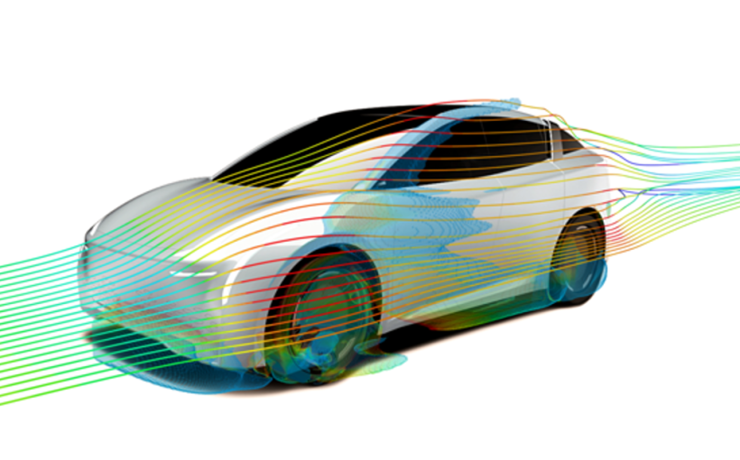
Artificial Intelligence is changing how we use computing power to solve complex problems. In Machine Learning, computers learn to make predictions and decisions based on data. This is why it is considered the most productive branch of modern Artificial Intelligence.

When design engineers model objects in 3D with CAD, they must decide on product shapes. This is why design engineers are interested in predicting the performance of a product.

Computational Fluid Dynamics (CFD) simulations are helping corporations with several design decisions. Examples are:

• the most aerodynamic shape of a car
• the most performing shape of a ship propeller
• the most efficient geometrical configuration of heat exchanger fins

So why isn't CFD on any engineer's desktop?

Two major drawbacks are hindering CFD's democratization:

• the time to complete a numerical simulation
• the skills required to use it at a reliable level (the so-called high-fidelity level).

How can Machine Learning and its newest evolution, Deep Learning, help CFD address these challenges?

In this article, we will describe the impact of the “Deep Learning Revolution” on engineers who need CFD but can’t keep on waiting for it.

Deep Learning is an enabler of democratization and acceleration of CFD. We will focus on

• why CFD should be accelerated;
• how was CFD traditionally accelerated;
• how is Artificial Intelligence now accelerating CFD simulation?

As a first example, let us illustrate the aerodynamics of F1 cars. Traditionally, computational aerodynamics of F1 cars is delegated to CFD specialists or aerodynamicists.

• The Why - Aerodynamicists want to select the best F1 car shapes for downforce and streamline structure. They access a portal, submit a batch job, and await the result. Meanwhile, a compute farm needs “number crunching” time before giving the results.
• The old How - The traditional approach is to increase the number of processors that crunch numbers to give answers faster. This solution comes at the cost of huge infrastructure investments, not to mention maintenance costs.
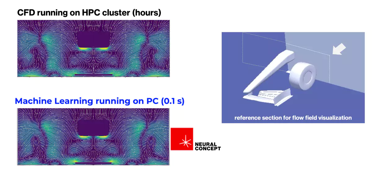
• The new How - Machine Learning and Deep Learning can speed up traditional CFD simulation not by a factor of 10 but by several orders of magnitude. This is shown in the figure.

This article will give you:

• a historical appraisal of the CFD speed challenge;
• basic knowledge of how contemporary machine learning works.

Before tackling the application of artificial intelligence to CFD, we will take you on a guided tour. We will show computational fluid dynamics deployed in various industrial sectors. This will help us understand why so much has been invested in CFD and its speed-up. Then, we will examine previous attempts to accelerate computational fluid dynamics.

Finally, we will explore neural network approaches with deep neural networks. Artificial Intelligence can boost CFD with neural information processing systems working on optimized training data.

Four use cases will show the application of deep learning to diverse applications of fluid dynamics and heat transfer in common.

‍

In Search of Engineering Answers

Let us take the example of F1 aerodynamics once again and think about a typical engineering prediction needed in F1 i.e. “what will be the aerodynamic downforce on the car”? The question allows us to explore the human brain’s performance, software reasoning like the human brain, and the outcome of data-driven Artificial Intelligence predictions.

We can think of it as “human” anything directly produced by the human brain (like an engineer issuing some guess on what will be the downforce in an F1 car) or by software like CFD that traditionally implements human physical knowledge of the world developed by physicists and engineers and implemented by mathematicians, computer scientists, and programmers. Physical knowledge is translated into partial differential equations, and equations are solved numerically by the computer.

How do humans approach the aerodynamic prediction of the F1 car?

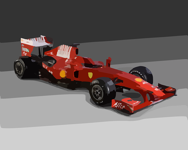
Intuition Is Real-Time but Biased; Computations Are Accurate but Slow

The human brain can intuitively guess a numerical value for downforce; this intuition will be immediate and more accurate for more experienced engineers. However, it will be so coarse that no helpful comparison can be made between the two car designs. The same happens (as experienced by the Author in the 90s) when making small manual shape modifications during expensive laboratory testing (velocimetry, wind tunnel testing). Even if initial successful modifications are obtained, it is difficult to predict a trend and to fine-tune solutions.

In contrast, CFD numerical simulation can produce accurate numerical values that can be used to compare different designs (hence, to explore the design space). This comes at the cost of heavy computational power and over-the-top skill requirements.

How to put together intuition and computation? Is there a computational intuition? Machine learning and deep learning architectures are a product of the human mind that exploit all the previously cumulated knowledge (stored as data) to learn quantitative predictions combining the speed of human intuition (a few milliseconds) and the accuracy of CFD simulation.

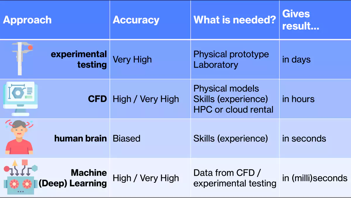
A most exciting side-product of the superhuman speed of deep learning is a superhuman performance in exploring the design space, i.e. the space of different design alternatives for a product in terms of shape or materials, in search for the optimum design that yields the maximum performance compatible with all the imposed constraints on the product (space, cost, weight, etc.).

This article will detail how deep learning techniques and neural networks are changing the game for CFD simulations in product design, making those simulations faster and more accessible to engineers and designers. Deep learning is a subfield of machine learning. It is quickly revolutionizing the field of applied CFD to product design because it can learn to recognize features such as edges, bends, and so on and give them physical meaning. But the real hands-on aspect of deep learning is that it can be delivered within intuitive apps driven by deep learning that do not require special skills from engineers. By giving simulation power to engineers, deep learning helps them to be more influential within their organizations.

The Relevance of CFD Simulation for the Industrial World

Computational fluid dynamics is a powerful tool that enables engineers to simulate and analyze the fluid flow and heat transfer in industrial applications. In this section, we will explore the importance of CFD in the industrial world, starting with an explanation of fluid dynamics and heat exchange within industrial contexts.

Fluid Dynamics and Heat Exchange in Industrial Applications

Fluid dynamics studies how fluids, such as gases and liquids, flow and interact with their environment. In industrial applications, fluid dynamics is critical for optimizing fluid movement processes. For example, fluid dynamics plays a vital role in the oil and gas industry in the drilling, transportation, and refining processes. In chemical processing, fluid dynamics is essential for mixing and reacting to different fluids. Fortunately for fluid mechanics and heat exchange specialists, those disciplines play a vital role in the "green transition" taking our economies by storm. Most renewable resources involve fluid mechanics aspects (imagine wind turbines or hydroelectrical plants) or heat exchange aspects often coupled with fluid mechanics, such as solar panels.

Fluid dynamics is also critical in designing and operating industrial equipment, such as pumps, valves, and turbines. Understanding fluid dynamics allows engineers to design equipment that maximizes efficiency and energy consumption. For example, in the automotive industry, the engine’s combustion chamber design and the flow of intake air and exhaust gases can significantly impact the engine’s performance and fuel efficiency. Cooling circuits for traditional or electrical engines guarantee their performance and reliability.

The topic of cooling circuits leads us to heat exchange, i.e. the thermal energy transfer between two or more fluids at different temperatures. In industrial applications, heat exchange is critical for heat transfer processes, such as power generation, refrigeration, and air conditioning. Efficient heat exchange is essential for reducing energy consumption and ensuring product quality. Heat exchangers are used in various applications, including power generation, chemical processing, and refrigeration. Understanding heat transfer allows engineers to design heat exchangers that maximize efficiency and reduce energy consumption.

Impact of CFD on Industrial Applications

CFD significantly impacts industrial applications, enabling engineers to optimize processes and equipment design. CFD simulations provide insights into fluid flow and heat transfer that are impossible with traditional experimental methods, not to mention mere human intuition.

Here are some examples of how CFD has been used in different industrial applications.

Aerospace Industry

CFD has become a vital tool in the aerospace industry for designing and optimizing aircraft and rocket engines. Also, with CFD simulation, engineers predict the behavior of fluids over the surfaces of aircraft and rockets at various flow regimes, providing valuable insights into aerodynamic performance and heat transfer.

• In aircraft design, CFD simulations can analyze and optimize the aircraft’s aerodynamics, including lift and drag, stability, and control. Engineers can evaluate the effect of design changes, such as altering the wing shape, fuselage design, or engine placement, to optimize the aircraft’s performance. CFD simulations can also be used to investigate flow separation, turbulent flows, and the formation of shock waves, which are critical factors in determining an aircraft’s stability and efficiency.
• In rocket engine design, CFD simulations are essential for predicting combustion and optimizing fuel injection and mixing processes. Engineers can analyze the fluid mechanics within the combustion chamber and nozzle, predict the engine’s performance, and optimize the design to improve thrust and fuel efficiency. CFD simulations can also investigate the flow of hot gases and exhaust products through the nozzle, affecting the engine’s efficiency.

Power Generation and Chemical Processes

CFD is essential to optimize the design of power plants, including combustion chambers and heat exchangers. CFD simulations have enabled engineers to reduce energy consumption and improve power generation efficiency. Engineers also use CFD to optimize chemical processes, including mixing chemicals and reactions. The engineer’s attention is focused on processes that, for example, minimize energy consumption and reduce waste.

Automotive Industry

CFD has been used to optimize the design of traditional engines and improve the aerodynamics of vehicles. It is also extensively used nowadays for EVs (electric vehicles). CFD simulations have enabled engineers to design more performing engines and cars with less air resistance, better climate control, and better thermal performance of batteries. The automotive industry is at the forefront of competitiveness and innovation, which explains the role of CFD and artificial intelligence in car manufacturing.

Other Transportation Industry: Naval and Yachting

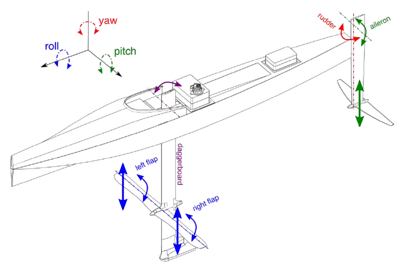
Since time immemorial, the naval and yachting industries have been aware of the importance of fluid mechanics for vessel performance, both for traditional dislocating hulls and for planing hulls (such as speed boats). An interesting analogy between the automotive and the naval industry is the strong presence of a racing sector (for instance, America's Cup) that allowed the testing of new technologies such as CFD in the 90s and early 20s before releasing the simulation software to companies more concerned with standard applications. Similarly, the Deep Learning revolution we will describe later focused on optimizing hydrofoil shapes for student races. Later, it was “ported” to more industrial and repeatable cases, such as large dislocating hulls.

Civil Engineering

CFD simulations had quite a slow start in this sector. However, nowadays, computational fluid mechanics helps civil engineers and architects. Since CFD simulations can predict the turbulent flows around the building and calculate the wind loads on the structure, this information can be used to optimize the design of the building and ensure that it is structurally stable and safe.

Wind loading on structures is also an essential consideration in the design of bridges, especially long-span bridges. CFD simulations can predict the wind flow around the bridge and calculate the wind loads on its structure. With this information, civil engineers can optimize the bridge’s design and ensure it is structurally stable and safe.

CFD simulations have also analyzed pedestrian comfort in urban environments, particularly in the “canyon effect” context. The canyon effect refers to the phenomenon where tall buildings on either side of a street can create wind channels that amplify wind speeds and create uncomfortable and potentially dangerous pedestrian conditions.

CFD simulations can predict the turbulent flows in urban canyons and assess the impact on pedestrian comfort. By simulating different wind conditions and building geometries, engineers can optimize the design of buildings and urban spaces to minimize the impact of the canyon effect and improve pedestrian comfort. In addition, CFD simulations can be used to assess the effectiveness of mitigation strategies, such as wind barriers, building setbacks, and vegetation. These strategies can help to disrupt the wind flow and reduce the impact of the canyon effect on pedestrians.

What Is CFD? Fluid Mechanics + Computer Simulation

CFD is a computational tool that enables engineers to simulate and analyze fluid mechanics and heat transfer, using numerical algorithms to solve fluid flow and heat transfer equations. The fluid flow equations are known as the Navier-Stokes partial differential equations. They represent the momentum balance and conservation of mass for Newtonian fluids.

We have seen in the previous chapter how CFD has become an essential tool in the industrial world, allowing engineers to optimize product design and processes.

CFD simulations provide insights into fluid flow and heat transfer that are impossible with the traditional experimental methods, simulating complex flow phenomena, such as turbulent flows, which are difficult to measure experimentally. Moreover, virtual testing with CFD is generally much less expensive than physical testing, all expenses considered (building and transportation of prototypes, laboratory set-up, storage issues of used prototypes).

A Short History of CFD Simulation

The history of CFD dates back to the early 20th century when the first attempts were made to solve the Navier-Stokes equations numerically.

However, it was not until the advent of computers in the 1960s that CFD simulations became feasible.

This involved breaking down the fluid domain into a grid of discrete points and using numerical methods to solve the governing partial differential fluid flow equations. The computational power of the computers available at that time limited the early CFD simulations. Only with the development of the finite element method (FEM) and the finite volume method (FVM) in the 1970s and 1980s did CFD simulations become more accurate and efficient.

The finite element method involves discretizing the fluid domain into a mesh of interconnected elements, while the finite volume method divides the fluid domain into control volumes. These latter methods allow for more accurate calculations of fluid flow and other physical phenomena.

The development of the first commercial CFD software packages in the 1980s was a significant breakthrough in fluid dynamics research. A pioneer of CFD was Prof. Brian Spalding, who created PHOENICS in the late 1970s, a then-revolutionary approach to simulate fluid flow and heat transfer in complex 3D geometries. In addition to PHOENICS, other CFD software packages have been developed, such as OpenFOAM, Fluent (now in the well-known ANSYS family), and STAR-CCM+ with its precursor STAR-CD, conceived by Prof. David Gosman at Imperial College London.

Despite their early stiffness and limitations (the Author took weeks to create the mesh and launch a simulation of an engine cooling circuit in the late 90s), all the latter software packages have continued to evolve and improve the application of computational fluid dynamics.

What Are the Risks in CFD Slowness?

What is the risk of delivering too slowly a CFD simulation? The risk increased as CFD became more and more relevant for business and came under the limelight. We will present an overview of the need for speed in the last decades and explain how Machine Learning arrived "just in time" in the last few years

The 80s and 90s

In the early 80s, the “analyst” (a specialized operator, mainly a scientist) had to spend weeks tuning their model. In the early 90s, slowly delivered CFD results meant that diagnostics and analyses arrived too late to be helpful in discussions involving engineering managers. To address this challenge, companies tried to adopt more direct ways to couple CAD (geometrical industrial representation of an object) to CFD, trying to overcome the considerable bottleneck represented by the construction of the computational fluid dynamics mesh. Another issue was the slowness of the solver, and a final bottleneck was the interpretability of results.

This decade produced, as an answer, at least three main innovations:

• Automatic meshing software (“meshers”) was produced and distributed independently or delivered within existing solver commercial packages.
• Parallel performance of the solver over several CPUs, with the gradual advent of multi-core CPUs.
• More realistic visualizations allowed final users to understand the fluid simulations and the “shadowed” geometry of the solid object.

The 00s

In the early 00s, the increasing complexity of engineering problems and the need for faster turnaround times led to a shift in the CFD industry. CFD analysts were now expected to deliver results within days or even hours instead of weeks, which meant they needed to develop new strategies to accelerate the solution of the Navier Stokes equations and other associated partial differential equations.

One of the most significant challenges during this time was the increasing size and complexity of the geometries involved, which made it difficult to solve problems efficiently. To address this challenge, CFD analysts turned even stronger than before to parallel processing, which allowed them to divide a large problem into smaller, more manageable pieces and solve them simultaneously. The availability of more powerful computing hardware and the development of new algorithms and solvers also contributed to faster simulations.

‍

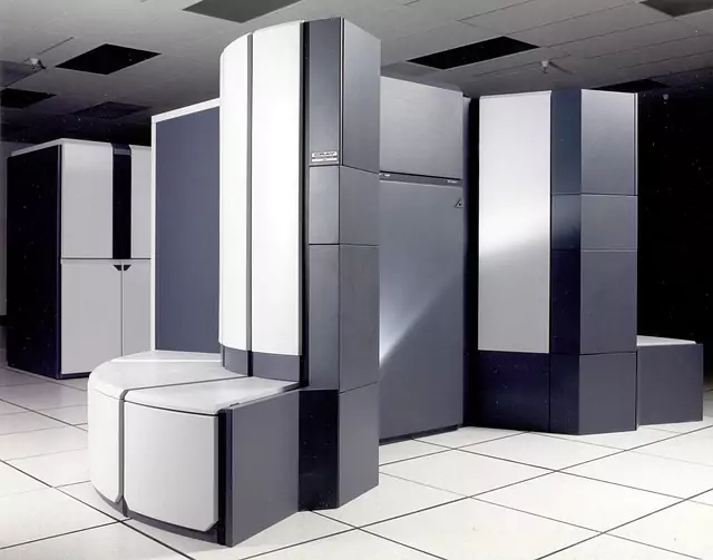
This era saw the definite consolidation of commercial CFD software, which became increasingly sophisticated and user-friendly, making it more accessible to engineers.

The 10s

In the early 10s, CFD analysts faced new challenges related to the increasing demand for simulation accuracy and reliability. As engineering problems became more complex, the need for high-fidelity simulations increased, which meant that simulations had to be run at higher resolutions and with more detail. This posed a significant challenge for CFD analysts, as higher resolution simulations required more computing power and longer simulation times. CFD analysts turned to new simulation methods, such as adaptive mesh refinement (AMR), to overcome this challenge. This is an example of how to focus computational resources where they are most needed. AMR works by automatically refining the mesh in areas where the solution changes rapidly while keeping the mesh coarse in areas where the solution is relatively smooth. This approach significantly reduces the computational cost of simulations, making it possible to run high-fidelity simulations more efficiently.

‍

Another significant and broader scope improvement was automatic meshing for very arbitrary meshes, going well beyond the initial tetrahedral approach.

1. Polyhedral Meshing: Polyhedral meshing is a technique that involves using polyhedral elements to fill most parts of the computational domain. For instance, the polyhedral meshing algorithm in STAR-CCM+ used various techniques to generate high-quality meshes shown to significantly reduce the computational cost of CFD simulations while maintaining high levels of accuracy and keeping the memory footprint under control.
2. Trimmed Cell Meshing: Trimmed cell meshing is a technique that generates high-quality meshes for complex geometries, such as automotive components or aircraft parts. The technique involves generating a high-quality mesh on the exterior surfaces of the geometry and then trimming (cutting) the cells in the geometry’s interior to match the boundary conditions. The technique has been shown to reduce meshing time and improve simulation accuracy, particularly for complex geometries with challenging internal features.

‍

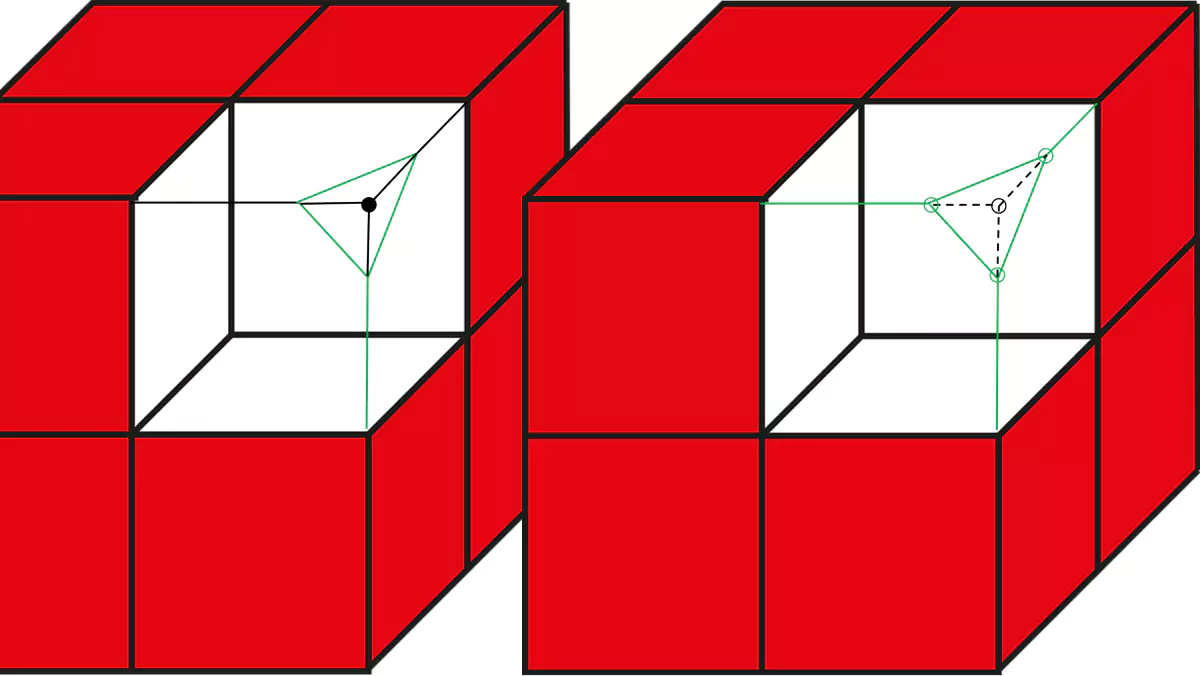
Both polyhedral and trimmed cell meshing have contributed to the evolution of CFD and its acceleration, enabling engineers to simulate increasingly complex geometries and reduce the cost of simulations. It has, however, to be mentioned that "meshing time" and "meshing memory" (RAM) are significant. Advances like parallel meshing, i.e. distributing it over several compute nodes, are making it faster but far from real-time.

The 20s

The demand for real-time CFD simulations has increased significantly in the last few years. This presents a challenge for analysts who need to optimize computing resources. Researchers are exploring new simulation techniques, such as reduced-order modeling (ROM) or model order reduction, which allows for real-time simulations by reducing the problem’s computational complexity. Model reduction works by constructing a reduced-order model that captures the essential features of the entire simulation while eliminating non-essential details. This approach significantly reduces the computational cost of simulations, making it possible to perform real-time simulations on less powerful hardware. This has been a significant step forward for CFD analysts, allowing them to perform simulations in real-time for engineering problems that were previously impossible to simulate in real-time.

Recent advancements in machine learning, specifically geometric deep learning, have led to new simulation techniques that go beyond model reduction and get rid of the previous parametrization constraints.

Geometric deep learning is a machine learning technique that can learn representations of geometric structures, such as those found in CFD simulations based on industrial 3D CAD geometries. CAD is "learned" as a 3D spatial representation of objects without manual parametrization.

This new approach has shown astonishing results in the simulation of complex engineering problems, providing even more opportunities for real-time simulations in CFD.

Why Accelerating Computational Fluid Dynamics?

In summary, CFD is a tool to enable engineers to simulate fluids and heat transfer in real-world scenarios, considering the realistic geometrical shapes (CAD) and complex physics of engineering processes.

To visualize and quantify fluid flow and heat transfer phenomena in industrial objects, the mathematical fluid flow and heat transfer models must be solved numerically. This involves solving partial differential equations that describe the conservation of mass, momentum, and energy.

However, Computational Fluid Dynamics simulations are time-consuming and computationally expensive. An example of computational effort is turbulence modeling, a critical aspect of many fluid flows that cannot be ignored. As said above, geometrical complexity and specific physics also play a role.

A core mathematical equation for fluid flows is the momentum equation, known as the Navier-Stokes partial differential equation. Flow, including turbulent flows, is solved using numerical methods such as the finite volume approach.

Solving the Navier-Stokes equations involves discretizing the fluid domain into many small elements and solving the partial differential equations at each element that are reduced to algebraic equations. This leads to creating a large system of linear equations, which must be solved using matrix inversion within an iterative numerical method. These methods are time-consuming, especially for large domains, making CFD simulations computationally intensive. In addition to matrix inversions, CFD requires numerous iterations of numerical methods to reach a converged solution. The number of iterations depends on the accuracy and the specific numerical method. This can lead to additional computational time, further contributing to the overall computational intensity of CFD simulations.

The computational cost of CFD simulations increases with the size of the fluid domain, the number of elements used for discretization, and the accuracy desired. For the sake of giving some qualitative indications without assuming we are stating a scientific law, we could roughly express the computational cost of CFD simulations as follows in big O notation: t = O(nᵈ log n), where t is the computational time, n is the number of elements used for discretization, and d is the dimension of the fluid domain. The spirit of the above equation is that the computational cost of CFD simulations increases exponentially with the number of elements used for discretization. Additionally, the logarithmic factor represents the cost of the numerical methods used to solve the partial differential equations, which increases as the number of elements increases.

Whatever the exact formula, there is universal agreement that CFD simulations are time-consuming due to the complex mathematical calculations involved in modeling fluid flow and the exponential increase in cost with the fluid domain’s size and the desired accuracy. A simulation with tens of millions of cells (finite volumes) could take, on a single-core CPU processor, several days to be completed. How to accelerate CFD simulations?

Accelerating Computational Fluid Dynamics: Simplified CFD Approaches

“Simplified” Computational Fluid Dynamics approaches involve reducing the complexity of the simulation to speed up the calculation time while preserving the appearance of a 3D CFD code with specific GUIs and CAD import facilitations for CAD designers.

These approaches include reducing the number of mesh points or spatial or temporal resolution. While these approaches can significantly reduce calculation time, they can also result in significant errors in the simulation results. These errors can often be dangerous and lead to incorrect predictions.

For example, “simple CFD” approaches can lead to significant errors when unsuitable turbulence modeling is used. Turbulence models are essential for accurately simulating turbulent flow behavior, but they add complexity to the simulation, increasing the calculation time. Thus, simplified CFD approaches often rely on less accurate turbulence modeling, such as a simple RANSE turbulence model, to speed up the calculation time.

However, unsuitable turbulence modeling can result in grossly inaccurate simulation results, particularly for turbulent flows. For example, the turbulent eddies transport momentum, heat, and other scalars in a turbulent flow, which cannot be resolved with a coarse mesh or a simplified turbulence model. In such cases, simplified CFD approaches can lead to significant errors in the predicted flow field, resulting in incorrect predictions of fluid behavior.

Moreover, simplified CFD approaches may also lead to the incorrect prediction of flow separation, which can have severe consequences for engineering design. Flow separation occurs when the fluid flow separates from the surface of an object, creating regions of low pressure that can cause drag, instability, and even failure of the object. Accurately predicting flow separation requires resolving the turbulence near the object’s surface, which is difficult to achieve with simplified CFD approaches.

In summary, while simplified CFD approaches can significantly reduce calculation time, they can also result in significant errors in the simulation results, particularly when unsuitable turbulence models are used. These errors can be dangerous and lead to incorrect predictions of fluid behavior, including flow separation, which can have severe consequences for engineering design.

Accelerating Computational Fluid Dynamics With Hardware

To get more accurate simulation results, CFD simulations require significant computational power and can take hours or even days to complete on a standard computer. As a result, there has been a push toward accelerating Computational Fluid Dynamics simulations through high-performance computing (HPC) systems and Graphics Processing Units (GPUs).

What are GPUs, and What is different from CPUs

A GPU, or Graphics Processing Unit, is a specialized microprocessor designed to perform complex mathematical and computational tasks required for rendering graphics and images. The GPU is designed to handle large amounts of data in parallel, making it highly effective for jobs that manipulate and process vast amounts of visual data. In contrast, the more traditionally known CPU, or Central Processing Unit, is a general-purpose microprocessor designed to handle various tasks, including executing program instructions, managing input/output operations, and performing basic arithmetic and logical operations. The CPU is optimized for sequential processing, meaning it executes instructions one at a time in a linear fashion.

‍

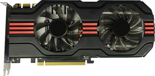
The primary difference between a CPU and a GPU lies in their architecture and design.

CPUs are optimized for single-threaded performance, which means they are designed to execute a single instruction at a time with high efficiency. In contrast, GPUs are optimized for parallel processing, which means they can run thousands of instructions simultaneously across many processing cores.

A typical standard CPU has a relatively small number of processing cores, ranging from 4 to 16, while a GPU can have hundreds or thousands of processing cores. The large number of processing cores in a GPU allows it to process vast amounts of data in parallel, making it highly effective for tasks that involve manipulating and processing large datasets, such as 3D modeling, image processing, and video rendering.

When choosing a GPU, you should consider the size of memory and the number of memory channels since they affect the GPU’s ability to store and process data. However, the first step in using a GPU for CFD simulations is "porting" the solver to a GPU platform since it is not just a plug-and-play operation. This involves rewriting parts of the solver’s code to take advantage of the GPU’s parallel processing capabilities, dividing the problem into smaller sub-problems. Once ported, the solver must be tested on the GPU to ensure it runs correctly.

HPC and Acceleration of CFD simulation

High-Performance Computing (HPC) systems use parallel computer clusters to perform complex calculations. These systems can significantly speed up CFD simulations by distributing the computational load across multiple computers with multiple CPUs or GPUs. HPC systems can range from a few computers to large data centers with hundreds of nodes. When used for CFD, HPC systems can provide significant speed-ups compared to traditional single-computer fluid simulation.

‍

The acceleration that can be expected from an HPC system depends on several factors, including the number of nodes in the cluster, the performance of the processors in each node, and the complexity of the Computational Fluid Dynamics simulation being run.

HPC systems are typically composed of several components, including:

• Nodes: The individual computers that make up the cluster.
• Interconnect: A high-speed network that connects the nodes and allows them to communicate.
• Storage: A large-scale storage system that can store the data required for the Computational Fluid Dynamics simulations.

What can be expected in practice from the HPC acceleration of CFD?

The figure shows the scale-up, i.e. the time it takes to complete a simulation on 1 processor, divided by the time it takes to run on a variable number of processors. Ideally, an HPC structure with “n” processors would allow CFD to run “n” times faster. Hence the ideal curve is a straight line.

‍

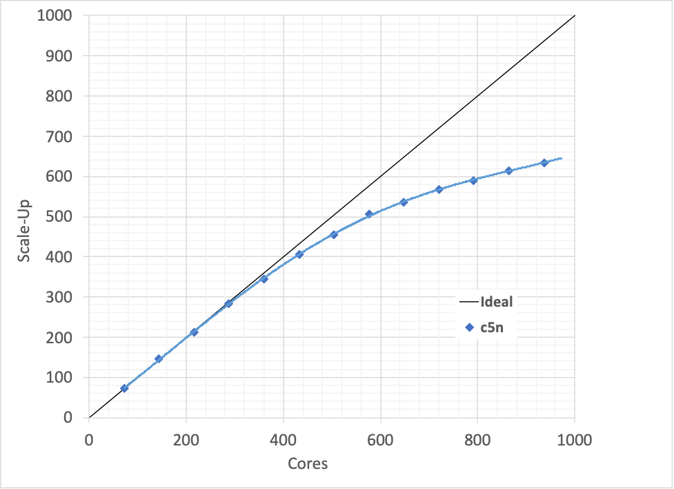
However, scale-up is less than ideal due to some of the above hardware and software factors. What is important to know for the design engineer is that scale-up comes at the cost of either internal resource investments or cloud computing rental.

In summary, HPC systems and GPUs can significantly accelerate Computational Fluid Dynamics by providing the computational power and parallel processing capabilities needed to perform complex calculations quickly.

While these approaches can be expensive regarding hardware and maintenance costs, they can provide significant benefits in speed and accuracy, making them important tools for engineers and scientists.

Beyond GPUs: TPUs

We will close the chapter on hardware by dedicating a section to TPUs.

TPUs (Tensor Processing Units) are specialized hardware accelerators designed by Google specifically for performing the machine learning computations we will discuss in the next chapter. TPUs were designed to accelerate the training and inference of neural networks and are optimized for machine learning linear algebraic operations.

TPUs differ from GPUs in several ways, such as how they handle memory. A bottleneck in large-scale machine learning applications can be the time required to move data between different memory spaces (LINK). GPUs typically have separate memory spaces for the CPU and GPU. This can lead to performance bottlenecks when moving data between the two. In contrast, TPUs have a unified memory architecture, meaning they have a single pool of high-bandwidth memory that all processing units can access.

TPUs can significantly reduce the time required to train large-scale neural networks. This can be important for applications that require large amounts of training data and complex models. Thus, using TPUs to train neural networks can allow you to train larger and more complex models than traditional CPUs or GPUs. TPUs are optimized for machine learning computations and are generally unsuitable for CFD simulations. CFD typically solves nonlinear partial differential equations by performing matrix manipulations with large systems of linear equations, which are tasks better suited to traditional CPUs in HPC or GPUs, as described in the previous chapters.

Accelerating Computational Fluid Dynamics With Machine Learning and Deep Learning

Machine learning algorithms can learn from data, making them ideal for improving the impact of CFD simulations by exploiting the data generated during simulations and stored in the companies’ data vaults. Machine Learning and Deep Learning are rapidly growing fields in computer science and artificial intelligence. While machine learning and deep learning involve teaching computers to make predictions and decisions based on data, their approach and complexity differ.

Machine Learning

Machine learning focuses on developing algorithms and statistical models that enable computers to learn from data and make predictions or decisions without being explicitly programmed. Machine learning algorithms can be divided into several categories. The most important for us are Supervised machine learning models.

Supervised machine learning algorithms are used when the data used to train the algorithm has labeled outputs. This machine learning type is used for classification and regression tasks, where the algorithm is trained to predict a categorical or numerical outcome based on input features. For example, a supervised machine learning algorithm could predict the likelihood of a customer defaulting on a loan based on their credit score, income, and other financial information. While machine learning has been used to solve many complex problems, it can be limited by the size and complexity of the data, and the model used. Deep learning is a subfield of machine learning that focuses on using deep neural networks to learn from and make predictions on complex data.

Another type of deep learning algorithm is deep reinforcement learning. Unlike supervised learning, deep reinforcement learning involves training an agent to make decisions based on feedback from the environment. In other words, the agent learns through trial and error by interacting with the environment and receiving rewards or penalties for its actions.

Neural Networks and Deep Learning Architectures

A neural network is a type of machine-learning model that is inspired by the structure and function of the human brain. A neural network consists of multiple layers of interconnected nodes, each representing a unit of computation. The nodes in the artificial neural network are organized into input, hidden, and output layers. The input layer receives the data used to make predictions, the hidden layers process the data, and the output layer provides the prediction. The nodes in a neural network are connected by pathways called weights, representing the strength of the connection between nodes. The weights in a neural network are learned during the training process, where the algorithm adjusts the weights to minimize the error between the predicted and actual outcomes.

Deep learning refers to using deep neural networks, which are neural networks with multiple hidden layers. The additional hidden layers allow deep neural networks to learn more complex representations of the data, which enables them to make more accurate predictions. Deep learning has achieved state-of-the-art performance in various tasks, including image classification, speech recognition, and natural language processing. Deep learning can learn from raw, unstructured data, such as images and text. This makes it well-suited for applications in which the data is complex and difficult to pre-process, such as image and speech recognition.

Neural Networks as Universal Approximators

A neural network is a machine learning algorithm that models the relationship between input and output data by learning a function that maps the input data to the output data. This function is typically denoted as “y = f(x)”, where x is the input data and y is the output data. The function f is determined by the weights and biases of the trained neural network, which are learned during training. Neural networks can approximate a wide range of functions, making them a powerful tool for solving complex problems. It has been shown that neural networks are universal approximators. Given a sufficiently large number of neurons and an appropriate activation function, they can approximate any continuous function to arbitrary precision with a single hidden layer (Cybenko, 1989).

The universal approximation theorem is based on the fact that a neural network with a single hidden layer can represent any function composed of a finite number of continuous functions. This is achieved using nonlinear activation functions, such as sigmoid, ReLU, or tanh, allowing the network to model complex relationships between input and output data.

Neural Network Activation Functions

The sigmoid function is commonly used as an activation function in neural networks. The sigmoid function maps any real number to a value between 0 and 1, which makes it useful for modeling probabilities or binary classification problems. The mathematical expression for the sigmoid function is f(x) = 1 / (1 + exp(-x)). The sigmoid function is nonlinear, meaning it can model complex relationships between input and output data. Another commonly used activation function is the Rectified Linear Unit (ReLU), which is defined as f(x) = max(0, x) where max(0, x) returns the maximum value between 0 and x. Thus, it can be visualized as a ramp.

The ReLU function is also nonlinear and particularly effective in deep neural networks (Nair & Hinton, 2010). The ability of neural networks to approximate any function has important implications for many applications. For example, neural networks have been used for speech recognition, image classification, and natural language processing, among other things. The neural network is trained in each application to learn a function that maps the input data to the desired output data.

Therefore, a neural network is a powerful tool for approximating complex functions between inputs and outputs. With the appropriate activation functions and a sufficient number of neurons, a neural network can approximate any continuous function to arbitrary precision, making it a universal approximator. This property has important implications for various machine learning and artificial intelligence applications.

Why Can a Neural Network be Fast?

Neural networks are often optimized for inference, making predictions, or classifying new data based on a trained model. The time of inference can be as low as 0.01 - 0.02 seconds.

How can inference be so fast?!

The speed of neural network inference is due to several factors. One of the most significant factors is that the neural network weights are fixed during inference. During training, the network weights were adjusted to minimize a loss function by iteratively computing gradients and adjusting the weights. However, once the training is complete, the weights are frozen, and the network can be used for inference. This means that the forward pass through the network, where input data is propagated through the network to produce an output, is much faster than during training. Training data-driven models used in machine learning algorithms is critical in determining their performance. Training can come from experimental or numerical simulation data, which can be used to train the algorithms and improve their ability to model turbulence and other complex fluid mechanics topics accurately.

Physics-Informed Deep Learning

Until now, we have talked about data-driven learning. In contrast, physics-informed learning involves incorporating physical laws and knowledge into the machine learning models to improve their accuracy and generalization ability. In other words, physics-informed deep learning combines the power of data-driven learning with the prior knowledge of physical laws, enabling the development of more accurate and robust models with fewer data points. For instance, physics-informed neural networks (PINNs) have been successfully applied in many fluid dynamics applications such as turbulence modeling, aerodynamic optimization, and flow control. PINNs can also be used to solve inverse problems where the objective is to estimate a fluid system’s unknown parameters or boundary conditions using limited training data.

Advanced Computational Fluid Dynamics Application: Large Eddy Simulation

Large eddy simulation is a turbulence modeling technique in Computational Fluid Dynamics but it still faces significant challenges. By using deep learning techniques, engineers can improve the accuracy of large eddy simulations and make them faster and more accessible. Physics-informed deep learning, for example, can incorporate physical constraints into large eddy simulations, resulting in more accurate turbulence modeling and predictions. The computational cost of large eddy simulation can be quite high, as it involves resolving the largest scales of turbulent motion while modeling the smallest scales.

The cost is primarily determined by the number of grid points in the simulation, which can be on the order of millions or even billions, and the time step size required to capture the flow dynamics accurately. In large eddy simulation, the large scales of motion are typically resolved directly on the grid, while the small scales are modeled using subgrid-scale models. This means that the grid resolution must be fine enough to capture the smallest scales of motion, which can be very small, leading to many grid points. Additionally, the time step size must be small enough to accurately capture the rapid changes in the flow field, which can also increase the cost of computations.

Use Cases for Deep Learning Techniques to Accelerate Computational Fluid Dynamics

We will now study four cases where Deep Learning techniques can accelerate traditional CFD approaches:

1. reaching optimal designs for heat exchangers;
2. performing better car aerodynamic predictions than other acceleration techniques;
3. helping study complex flow structures such as in turbomachinery (case 3);
4. contributing to project risk mitigation in civil engineering by accelerating fluid dynamics predictions.

Use Case 1 - Heat Exchangers and Machine Learning for Generative Design

Heat exchangers are critical components in many engineering systems that transfer thermal energy between fluids or gases. Their importance lies in their ability to improve energy efficiency and performance, reduce costs, and increase the lifespan of machinery. In the automotive industry, heat exchangers play a crucial role in regulating the temperature of various components, such as engine coolant, transmission fluid, and air conditioning refrigerant.

The design of heat exchangers involves a complex interplay of fluid dynamics, thermodynamics, and materials science. Engineers must consider factors such as flow rate, pressure drop, heat transfer coefficient, and fouling resistance. These parameters can be optimized through various methods, such as Computational Fluid Dynamics simulations, experimental testing, and advanced manufacturing techniques.

Even minor improvements in heat exchanger design can significantly impact energy efficiency and performance. For example, reducing the thickness of heat exchanger fins or increasing the surface area can enhance heat transfer and improve overall system efficiency. Additionally, utilizing advanced materials such as graphene or nanotubes can further increase heat transfer rates and reduce the weight and size of the heat exchanger.

The design and optimization of heat exchangers is a crucial aspect of engineering and is critical in many industries. Advancements in heat exchanger technology will continue to be essential in improving energy efficiency, reducing costs, and increasing the lifespan of machinery.

However, designing an efficient heat exchanger can be challenging since the number of parameters describing the heat exchanger geometry can quickly rise as the design becomes more complex. Product design engineers can only afford to explore a limited portion of the design space because of the growing costs of simulations.

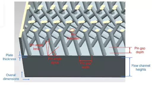
The engineering team of PhysicsX collaborated with Neural Concept to overcome this challenge by developing a surrogate model that can predict the performance of various heat exchanger designs with different topologies in real time. Starting from CAD and CAE training data, the surrogate model (NCS) can accurately predict the overall efficiency of the system, as well as temperature and pressure drop at the outlets. Engineers can interact with the heat exchanger designs in real-time, iterate efficiently between different geometries and topologies, and improve the system’s performance.

In addition, the model can predict the flow inside the volume, providing engineers with a better intuitive understanding of the phenomenon. The optimization library of Neural Concept was used on top of the surrogate model, bringing substantial improvements to the final design. The successful results of this collaboration encouraged PhysicsX and Neural Concept to continue working on various topics, providing a game-changer for CAD and CAE engineers, shortcutting the simulation and design optimization chain, and considerably improving products’ performance.

Use Case 2 - Utilizing Machine Learning to Enhance Performance of Next-Generation Vehicles

This case study shows the performance of a real-time predictive model for external aerodynamics that can be applied to production-level 3D simulations. The benchmark case developed between PSA and Neural concept aimed to accelerate design cycles and optimize the performance of next-generation vehicles.

The study compared deep learning fluid simulation with Gaussian-Process based regression models, specifically tuned for production-level simulations. The deep learning fluid simulation Geometric CNN mode was found to have much broader applicability than Gaussian Process. Furthermore, it does not require a parametric description and can outperform standard methods by a large margin.

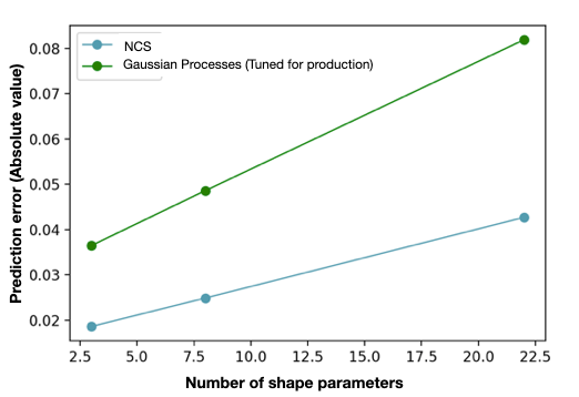
NCS is a data-driven machine learning software that learns to recognize 3D shapes (CAD) and how they relate to CFD (aerodynamics) results. NCS emulates high-fidelity CFD solvers, with inference (prediction) feedback in 0.02- 1 seconds following a CAD input compared to minutes to hours (or even days) for a CFD solver, which also needs mesher software to handle CAD. Engineers can use NCS to explore design spaces interactively or automatically with generative design algorithms.

NCS bridges the gap between designers and simulation experts, reducing lengthy iterations between teams to converge on a design solution.

This allows for a significant acceleration in product design and supports teams in the most complex engineering challenges.

Use Case 3 - Turbulence Modelling Development with Machine Learning

Applied fluid mechanics faces the challenge posed by our limited understanding and poor prediction capability of turbulence flows, resulting in industrial uncertainty in CFD for various aerospace and power generation applications.

The HiFi-TURB project, coordinated by NUMECA (now Cadence), aims to address such deficiencies through an ambitious program. HPC has enabled the development of turbulence models through Artificial Intelligence and Machine Learning techniques applied to a database of high-fidelity, scale-resolving simulations. NCS was used to analyze large amounts of 3D scale-resolving fluid simulation data.

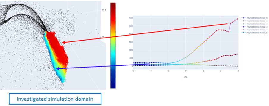
NUMECA used Neural Concept’s Geometry-based Variational Auto-Encoders* to gain insights into the correlation between statistically averaged flow variables. The machine learning model compressed the data physically into ‘embeddings’ and then reconstructed the original input with high accuracy.

The figure shows an example: the colors of the symbols on the 2D plot correspond to the value of the ‘embedding’ and are the same in the 3D view (left) and in the 2D plot (right). Points of the same color have the same value for all the considered physical quantities. The 3D view colored by the embedding value gives us one global statistical representation for several physical quantities over the investigated domain. Both plots provide a new perspective on the flow behavior via the machine learning model. The figure shows snapshots of the views used in the Graphical User Interface.

(*) Appendix to the Use Case - Geometry-based Variational Auto-Encoders (VAEs) is a machine learning model, a variation of traditional auto-encoders, i.e., neural networks that aim to learn a compressed input data representation. In contrast to traditional auto-encoders, Geometry-based VAE uses a geometric interpretation of the compressed data space. The VAE first maps the input data to a lower-dimensional latent space called an “embedding.” The embedding is then used to generate a reconstructed version of the input data. This geometric interpretation allows for more precise and meaningful representations of the input data. Geometry-based VAEs are particularly useful for analyzing and compressing high-dimensional data, such as 3D shapes or complex fluid flow fields like the ones seen before.

Use Case 4 - Deep Learning Fluid Simulation for Civil Engineering

Orbital Stack’s integration with Neural Concept’s machine learning software has revolutionized the design process for civil engineering.

Previously, designers had to wait up to 10 hours for each design iteration to be processed, significantly slowing down the design process. However, with Neural Concept’s model (NCS) now embedded in Orbital Stack’s CFD offering, the iteration time has been dramatically reduced to just a few minutes, exploiting vast amounts of training data from experiments and CFD simulations owned by Orbital Stack.

This means that designers can run multiple iterative simulations in a shorter period, significantly improving their workflow. Additionally, they can select the optimal version of their project while limiting environmental impacts on the design, ensuring that the design is efficient and sustainable.

By providing design iterations at different stages of the workflow, the software enables designers to optimize the performance of their designs and identify potential risks much earlier in the process. This allows for faster design cycles and provides reliable airflow analysis on demand. As a result, the final design’s performance and sustainability are improved, and designers can explore limitless design possibilities.

‍

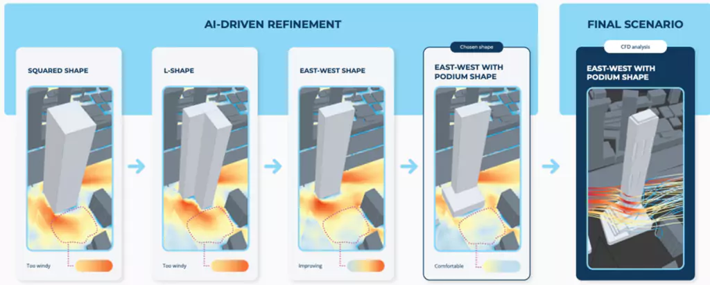
Integrating Orbital Stack and NCS has also streamlined the wind-tunnel analysis process. Thanks to deep learning fluid simulation, designers can validate their design optimization and meet regulatory requirements without surprises. The combination of Orbital Stack and NCS has significantly improved the design process, saving time, increasing performance, and promoting sustainability.

Conclusion

In conclusion, machine learning and deep learning are transforming the field of Computational Fluid Dynamics and have the potential to revolutionize the way engineers and designers approach fluid flow analysis and simulations.

Whether you’re working on designing better turbines, improving fluid mechanics research, or analyzing turbulence, machine learning can help you achieve your goals faster and more effectively.

By incorporating machine learning models into computational fluid dynamics, you can get faster accurate predictions of fluid behavior.

This can lead to better designs and understanding of complex fluid flows, ultimately leading to more efficient and effective engineering solutions.

‍

Quoted Papers

Cybenko G.V., (1989) “Approximation by superpositions of a sigmoidal function”. Mathematics of Control, Signals and Systems, 1989, vol. 2, p. 303-314.

Nair, V. and Hinton, G.E. (2010) “Rectified Linear Units Improve Restricted Boltzmann Machines”. Proceedings of the 27th International Conference on Machine Learning, Haifa, 21 June 2010, p. 807-814

‍

Cover image: courtesy of Applus+IDIADA