3D Convolutional Neural Network (3D CNN) — A Guide for Engineers

A 3D Convolutional Neural Network (3D CNN) is a deep learning architecture that extends the concept of pattern recognition from two dimensional data to three-dimensional inputs. Instead of processing data in height and width only (like 2D CNNs), 3D CNNs operate over height × width × depth (input volume), making them ideal for volumetric data (e.g., CT scans, CAD models, CFD simulations) or time-series of images (video). This added depth dimension allows the network to detect patterns and correlations across multiple slices or frames, enabling engineers to extract richer and more context-aware features for tasks such as simulation acceleration, defect detection, and complex product design.
Artificial Intelligence (AI) and Deep Learning (DL) revolutionized how we approach engineering problems. The revolution took off in computer vision and speech recognition; now it is spreading to product design. One of the most exciting progresses in DL is the Convolutional Neural Network (ConvNet). Recent research has opened the way for implementing even a 3D Convolutional Neural Network. 3D CNNs are key enablers for the revolution in engineering; empowering product design engineers with high-end simulation capability. SO 3D CNNs are an extension of traditional Convolutional Neural Networks, designed to handle data with spatial dimensions including height, width, and depth.
In this article, we will introduce the concept of 3D CNNs and explore its business relevance, particularly in fields like medical imaging . We will start with a case from the automotive industry.
In this article you will learn:
- Preliminary Case History: Better Competition with 3D Convolutional Neural Network
- How to Support Product Design?
- Can My Company Use AI to Predict Designs?
- Why 3D Convolutional Neural Networks Matter for Engineers
- Learning - in Humans and Artificial Agents
- Training Humans
- Introduction to Deep Learning Training
- Technical Aspects of DL Training
- Predicting with DL
- Prediction & Regression Speed
- What Are Classification and Regression?
- Practical Examples: Cats Vs Dogs & House Prices
- Classification and Regression in ML
- Deep Learning and 3D CNN Architecture
- How Neural Networks Learn
- aaaa
- The Goal of Deep Learning
- 3D CNNs: Classification
- 3D CNNs: Regression
- Training the Neural Network
- Training: Loss Fuctions
- Training: Loss Gradient
- The Building Brick: The Artificial Neuron
- Model for the Single Physical Neuron
- The Artificial Neuron
- Building Blocks of the Artificial Neuron
- Core Operation in the Artificial Neuron
- From a Single Neuron to a Neural Network
- Neural Network Training
- Neural Network Training Data
- Loss Functions
- How Does a 3D Convolutional Neural Network Work?
- Layers & Feature Maps
- Max-Pooling Layers
- Fully Connected Layers
- Convolution in Detail
- The Mathematics of Convolution
- Application to Image Processing
- Advantages of Convolution
- What is a gCNN?
- Advantages - gCNN
- More on gCNN
- What are Euclidean and Non-Euclidean Distances?
- Euclidean Distance
- Non-Euclidean Distance
- Cat Example
- 3D Convolutional Neural Network Applications
- Medical Imaging
- Video Classification
- Autonomous Driving and Image Classification
- Geoscience
- Material Science
- 3D CAD Models
We will explain basic concepts of this technology for readers without an AI background, progressing to advanced applications, including training and validation sets, as well as model building . The goal is to understand how neural networks enable AI to “learn” 3D CAD shapes.
The learning process aims to create a predictive model that forecasts engineering behavior, like a car’s aerodynamics, using related data. By the end, engineers will grasp this technology’s basics and be equipped to influence their organization positively in product design.
Preliminary Case History: Better Competition with 3D Convolutional Neural Network
This case involves Tier 1 suppliers providing automotive parts to OEMs, based on the author’s experience as an engineering director across four lines: passenger cars, luxury, trucks, and aftermarket. The process begins with an OEM’s RFQ to multiple suppliers, competing from design to manufacturing. Recently, OEMs and suppliers shifted from mainly using product simulation to fix issues to comparing design options and exploring solutions.
Two major challenges with traditional, high-fidelity simulation (CAE) are still in 2025:
- how to make simulation technology accessible to all engineers without extensive infrastructure and training
- how can we enable all engineers to interactively explore several design options?
An early engineering predictive capability accessible to R&D, product design, and sales teams could give sales engineers a competitive edge in RFQs and customer relationships.
Next, we review tools that provide evidence that products are innovative, cost-effective, and meet performance targets.
How to Support Product Design
The most effective way to support product design is to combine engineering expertise with intelligent, data-driven tools capable of tasks such as image segmentation to predict performance and verify compliance before a single part is manufactured.
How can we demonstrate that a product complies with targets and constraints before manufacturing?
There are three possible approaches:
- The first strategy is copying previous product designs, but this isn’t sustainable long-term due to issues like win-lose dynamics, mistrust in performance, and poor regulatory adaptation.
- The second involves costly, time-consuming testing, prototyping, and CAE simulations, requiring significant resources and investment amid fierce competition.
- The third, most innovative approach, uses DL to recycle solutions into predictive models. This enables organizations to demonstrate product capabilities quickly with real-time, deployable data-driven neural network models.
Once a real-time solution is available, it is immediate to consider the next step of implementing it in an iterative design process, thus reaching your product’s desired objectives faster, such as reduced weight, better heat dissipation, and better energy efficiency. The iterative design process can be automated and operated by humans or embedded in a generative design approach.
Can My Company Use AI to Predict Designs?
Entering the world of AI-driven simulation for product design is not as complicated as it may seem.
The two key ingredients you need to get started are a business case and data:
- A business case is simply the need to be competitive and innovative to attract customers or prospects
- Data are generated whenever your company designs CAD and performs CAE simulation or testing
For instance, you must deliver a product in 8 weeks instead of 6 months. That’s your business case. And you have data from the last 2 years, during which you’ve created 4 product concepts that can be used to train your AI.
In the following, we will provide a more detailed explanation on how prediction arises from data, particularly in the context of video analysis . But regarding practical deployment, the Neural Concept platform, which is based on 3D CNNs, already empowers CAE engineers and data scientists to build CFD surrogates and deploy them to designers.
Why 3D CNNs Matter for Engineers
In short, 3D CNNs approaches can improve accuracy and performance compared to traditional models, resulting in a competitive advantage and increased market share for your company.
Please note that all the following technical details aim to satisfy your curiosity about the inner workings of Deep Learning tools such as Neural Concept platform. Still, we assure you that the practical usage of the Neural Concept platform for AI-assisted engineering prediction has no prerequisite AI, data science or computer science skills.
In the next chapters, we will first review how 3D CNNs work, exploring such topics as classification and regression (two forms of prediction), and then move on to the architecture of 3D CNNs with more details on its building blocks, such as artificial neurons and filters.
Learning - in Humans and Artificial Agents
We will first give an overview of the AI training process, a key passage towards an actionable AI for designers.
There are three main types of AI learning. We will focus on supervised training, i.e. training with labelled data to predict labels for new examples.
Two other approaches are
- unsupervised training (finding patterns in unlabeled data) and
- reinforcement training (training through interaction with an environment).
A model is trained to perform a task based on labelled examples in supervised training. This process can occur with humans and artificial intelligence (AI) systems. The differences between human and artificial training can provide insight into the strengths and limitations of AI. Let's use image classification to compare supervised training; in this task, the deep learning model is trained to identify the class of an image (e.g., dogs, cats, etc.) based on labelled examples of images.
What about humans?
Training Humans
Humans learn through experience and observation, recognizing objects in images by repeated exposure to labeled examples. From early childhood, this process involves real objects and verbal interaction. It is time-consuming and memory-intensive, but humans benefit from understanding context and applying prior knowledge to identify objects in new images.

Introduction to Deep Learning Training
Deep learning systems can perform tasks much faster and more efficiently than humans. However, they are trained to carry out specific tasks without truly understanding the meaning or context behind their actions. We aim to automate engineering tasks that can be easily translated into mathematics and extract data from past experiences, such as design, laboratory testing, and CAE simulations.
It’s important to recognize that deep learning techniques have certain limitations. Unlike humans, these systems do not understand the context and meaning of images. Instead, they use the features and characteristics they’ve learned from labelled examples to make predictions. This means they may not generalize well to new or unseen images.
Technical Aspects of DL Training
Deep learning (DL) systems can be trained on large datasets of labelled images to learn the features of each object class quickly. The process involves adjusting mathematical connections, called “weights,” in the model (a neural network). This minimizes the error between predicted and actual class labels using algorithms such as gradient descent, enabling the DL system to learn much faster than a human could.
Predicting with DL
Deep learning systems can make predictions much faster than humans, achieving superhuman performance. For instance, they can process images and produce classification results in real time, whereas a person would need far longer to identify each image. In a multi‑class classification problem, the model assigns a probability to each possible category and selects the one with the highest score.
When dealing with video files, the model evaluates each frame (or groups of frames) and aggregates the results to classify the sequence as a whole. This allows recognition of actions, events, or objects across thousands of frames within seconds.
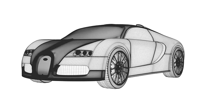
The speed advantage of DL is particularly evident with complex industrial designs. Predicting the temperature on the surface of a complex industrial geometry given its operating conditions is precisely the type of data-driven engineering prediction that the Neural Concept platform specializes in. Such predictions are known as regression.
Prediction & Regression Speed
The challenge can be not about classification but regression, i.e., predicting a number, such as in the following question - what is the aerodynamic coefficient of this car, given the image of the car?
What is the aerodynamic performance of this car, including pressure and velocity around and on its body, to calculate drag and downforce?
The answer can be via
- traditional software (CFD) simulating fluid mechanics and turbulence or
- AI trained on such data to predict values based on geometry. The AI approach can achieve superior performance compared to software coded by humans based on physics. 3D CNNs predictions can be several orders of magnitude (from 1,000 to 1,000,000) faster than traditional computational software such as CAE, based on physical knowledge of aerodynamics and industrial geometries such as cars.
What Are Classification and Regression?
Classification and regression are two common types of supervised machine learning (ML). More precisely, in a classification task, the goal is to predict a categorical label for a given input data. In a regression task, the goal is to predict a continuous value for a given input.
Practical Examples: Cats Vs Dogs & House Prices
Let’s start with a simple example to understand the difference between classification and regression. Imagine you have a dataset of images of cats and dogs, and you want to train an ML model to predict whether each image is a cat or a dog. This is a classification task where the output is a label (“cat” or “dog”). The input is the image, and the output is a binary label (“0” for cat, “1” for dog). The model learns patterns, like fur and whiskers, to predict the label.
Now, consider a dataset of housing prices. You want to predict a house’s price based on size, number of bedrooms, and number of bathrooms. This is a regression task with a continuous output. The input is the features, and the output is the house price. The model learns patterns, like larger size and more rooms, to predict prices.
Classification and Regression in ML
In supervised ML, tasks are typically split into two main types: classification, which predicts discrete categories, and regression, which predicts continuous numerical values. Both approaches train a model on labelled data to learn the mapping from inputs to outputs.
What is classification in Machine Learning?
Classification is a type of supervised learning that predicts a categorical label for a given input. Each sample belongs to exactly one class, which can be binary (e.g., cat or dog) or multi-class (e.g., red, green, blue).
The model is trained on a labelled dataset (pairs of input data and category label) to learn how to map new inputs to the correct class.
Key evaluation metrics include:
- Accuracy – proportion of correctly classified samples.
- Precision – proportion of predicted positives that are correct.
- Recall – proportion of actual positives correctly identified.
- F1 score – harmonic mean of precision and recall.
A confusion matrix is often used to visualise performance, showing true positives, false positives, true negatives, and false negatives. Correct predictions appear on the diagonal; errors are in the off-diagonal cells.
What is regression in ML?
Regression is a type of supervised learning that predicts a continuous numerical value for a given input, such as temperature, fuel efficiency, or price.
The model is trained on a labelled dataset (pairs of input data and numerical targets) to learn the relationship between the features and the continuous output.
Key evaluation metrics include:
- Mean Squared Error (MSE) – average squared difference between predictions and true values.
- Mean Absolute Error (MAE) – average absolute difference between predictions and true values.
- R-squared (R²) – proportion of variance in the target explained by the model.
A higher R² generally means a better fit. However, it must be interpreted with other diagnostics (e.g., residual plots) to detect overfitting or poor generalisation.
Deep Learning and 3D CNN Architecture
A 3D CNN refers to neural network architectures with multiple layers that can learn hierarchical data representations. Each layer learns increasingly complex spatial features of data. These 3D CNNs can then be used for various tasks such as classification, regression, or generation. Each type of layer has a definite function. 3D CNNs process volumetric data and are specifically designed to capture spatial and temporal dependencies. 3D CNNs utilize 3D convolutional layers that apply three-dimensional filters to scan the input data. For instance, 3D CNNs achieve better accuracy in analyzing temporal relationships in video data compared to 2D CNNs, which treat video frames as separate images.
Example Layers in a 3D CNN
For example, the max-pooling layer is a “downsampler” for feature maps. 3D convolutional layers typically reduce the size of feature maps through pooling layers, which operate in three dimensions.
A feature map is generated by convolving a filter over an image reducing its spatial size and computational burden. Another form of pooling is global average pooling.
How Neural Networks Learn
A neural network includes interconnected processing nodes - artificial neurons. Let’s have a deeper look at the connection between neurons and learning. How can they possibly learn? The key to the approach shown here (supervised learning) is to have examples to learn from.
In DL, neurons are organised into layers (this is the “depth” of DL).
Neurons in the first layer process the input, and the output from one layer is used as input for the next layer, and so on until the output from the final layer fairly represents the prediction.
Furthermore, each layer is trained to learn a different data representation. For example, in image classification, the first layer may learn to recognise edges and basic shapes, and the next layer may learn to recognise more complex shapes, and so on, until the input reaches the final layer. It transforms into a high-level representation to make a prediction or classify images.
How Does Training Work?
Neurons’ weights in DL neural networks are trained using backpropagation. Backpropagation updates the weights based on the error between the predicted output and the ground truth label. The error is propagated backwards (hence the name of backpropagation!) through the network, and the weights are adjusted to reduce the error.
This process is repeated until the error reaches an acceptable level.
If ŷ is the prediction for a given input x, the error between the predicted output and the true label y is expressed by formulas such as:
E = (ŷ - y)²
A training process aims to minimize this error by adjusting weights and biases in the network. The weights are optimized with algorithms such as gradient descent, adjusting the weights in the direction of the negative gradient of the error E.
What is the Goal of Deep Learning?
Deep learning aims to build systems that create their own internal models of data rather than relying on rules defined by humans. Through training, millions of model parameters are adjusted. These models capture relationships in data that are too complex to specify manually. The objective is not to mimic how people learn but to develop methods that can solve problems where explicit programming is impossible because the patterns are unknown or too numerous to enumerate.
3D CNNs: Classification
3D CNNs are deep learning models used in various applications, such as computer vision or medical imaging. For instance, the application of 3D CNNs in the medical imaging computer vision domain allows for better detection of tumors, lesions, and other abnormalities.
In these cases, we want AI to learn how to react to inputs rather than programming the AI according to a predetermined pattern. The outcome of this learning process is a predictive model. The predictive models emerging from the 3D CNN framework are designed to process and analyse data with a temporal dimension, such as videos. 3D CNNs can be used for processing 3D point cloud data from LiDAR sensors for object detection and semantic segmentation tasks in robotics and autonomous vehicles.
Computer "vision" means that the 3D CNN can learn spatial relationships within the data and extract features that can be used for tasks such as classification or segmentation. The goal is to assign a semantic label, such as "road", "building", "vehicle", etc., to each pixel in the image, providing a detailed understanding of spatial information in the scene. A recent innovation is applying a 3D convolutional neural network to deep learning models to capture how simulation software can associate accurate engineering predictions to CAD designs, also with predictive uncertainty.
3D CNNs: Regression
Earlier we mentioned using a 3D CNN to deep learning models to capture how software can associate accurate engineering predictions with CAD designs.
If the 3D ConvNet is trained on CAD geometries associated with CFD results, it will perform a regression rather than a classification task. In this scenario, the input to the network would be the CAD geometry, and the output would be the corresponding CFD result.
The 3D ConvNet would learn to map the input CAD geometry to the output CFD result based on the data for training. This could be useful in problems where the goal is to find the optimal CAD geometry, where performance comparison is carried out by CFD or its ConvNet surrogate.
The CFD surrogate works by extracting features from the input CAD geometry using 3D convolutions and processing these features through multiple layers to produce the final output. The network weights are updated during training to minimise the difference between the predicted CFD results and the ground truth CFD results.
Thus, it becomes possible to envisage (and reach) very ambitious objectives, such as coupling the neural network regression capability to a geometrical shape to optimize, leading to generative AI engineering (creating new shapes within the AI software without the need for third-party tools).
Training the Neural Network
During training, the network weights are updated to minimise the difference between the predicted CFD results and the CFD results: this is done using a loss (or error) function, which measures the error between the predicted CFD results and the ground truth CFD results.
Training: Loss Functions
A common loss (or error) function used in regression tasks is the mean squared error (MSE) loss. The loss (error) measures the average difference between the predicted CFD results and the CFD results.
The goal of training is to minimise this value and is expressed as
Loss = (1/N) * Σᵢ (ŷᵢ - yᵍᵗ)²
where
- N is the number of samples in the training set,
- ŷᵢ is the predicted CFD result for the iᵗʰ sample, and
- yᵍᵗᵢ is the ground truth ("gt") CFD result for the iᵗʰ sample.
The summation runs over the dummy index i for samples from 1 to N.
Whatever the exact mathematical form, the network weights are updated using an optimisation algorithm such as stochastic gradient descent (SGD) to minimise the loss.
Training: Loss Gradient
The loss gradient is computed using backpropagation, which allows the network to update the weights in the direction of minimal loss. The weight update rule for SGD is given by:
w' = w - η * ∇ Loss
where w is the weight, η is the learning rate, and ∇Loss is the loss gradient along the weight.
The learning rate η determines the step size at which the weights are updated, and it is a hyperparameter that must be chosen carefully:
- a high learning rate can cause the network to converge quickly, but it may not find the optimal solution
- a low learning rate can provide a more accurate solution but may take longer to converge.
The Building Brick: The Artificial Neuron
The Artificial Neuron is the basic building block, a sort of atom, of Artificial Neural Networks (ANNs), which are modelled after the structure and function of biological neurons in the human brain. ANNs are defined as "computational models that simulate how the human brain processes information".
We restrict this ambitious definition to a more specific one: a useful ANN for engineers is "a computational model that reproduces some specific functions of the brain, or software produced by humans, used in engineering, to assist humans with superhuman speed".
Model for the Single Physical Neuron
The human brain is complex, processing vast information to facilitate interaction with surroundings. Neurons, specialized cells transmitting information, are crucial. They receive, process sensory data, and send signals via electrical and chemical means. Interconnected neurons form networks that process info in parallel, with connection strength influencing their firing likelihood.
Mathematical models of neurons and neural networks have been developed to understand how the brain processes information. These models can predict neuron response to stimuli and show relationships between neurons. A simple mathematical model of a neuron is an artificial neuron consisting of inputs, weights, and an activation function that converts inputs into output.
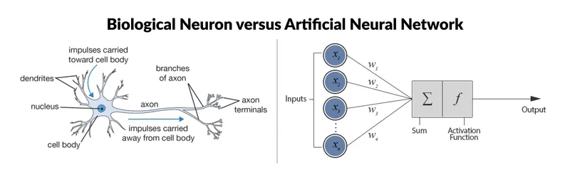
The Artificial Neuron
For our engineering purposes, artificial neurons serve as simplified models inspired by biological neurons, used as building blocks for complex functions like human brain simulations or software. Perceptrons are mathematical functions that process inputs to produce outputs. We do not aim to replicate biological neurons precisely - just to use them as a basis for artificial learning.
Building Blocks of the Artificial Neuron
Artificial Neurons have three components:
- inputs x; they are the signals the neuron receives from other neurons in the network.
- weights w; values that determine the strength of the input signals
- and an activation function f, a mathematical operation that determines whether the neuron will fire, or generate an output signal y, based on the input signals x and weights w.
So we imagine something like
y=f(x, w, b)
where the bias term b could represent other parameters.
The inputs to an artificial neuron are multiplied by their corresponding weights, and the results are then summed.
Core Operation in the Artificial Neuron
The artificial neuron mathematics can be represented as
y = w • x + b
where “b” is the bias term, and “y” is the resulting sum of all weighted inputs.
This weighted sum is passed through an activation function f, as mentioned above, which determines whether the neuron will generate an output signal. This function is usually non-linear, such as a sigmoid or rectified linear unit (ReLU), allowing the network to model complex relationships between inputs and outputs.
The function can be a sigmoid function:
f(z) = 1 / (1 + e⁻ᶻ)
or a rectified linear unit (ReLU) function:
f(z) = max(0, z).
From a Single Neuron to a Neural Network
Artificial Neurons are the building blocks of ANNs and can be connected to form more complex models. For example, multiple artificial neurons can be connected to form a layer of a neural network, and multiple layers can be stacked to form a deep neural network. In a neural network, each neuron receives input from multiple neurons in the previous layer, and the output from each neuron in one layer is used as input to multiple neurons in the next layer.
Neural Network Training
Training a neural network involves recognising parameters to minimise errors between its predictions and outputs. The network is provided with input + output data called training data. The training aims to find the best parameters that allow the network to predict the outputs for these data correctly. This is achieved through ML algorithms, which adjust the parameters based on the difference between the predicted and actual outputs.
Neural Network Training Data
More training data of better quality is crucial for training neural networks successfully. More data means better learning, but data quality is important to avoid biased or noisy results. Balancing underfitting and overfitting is another challenge, where the network may be too simple or too complex, resulting in poor performance. Techniques like regularization, early stopping, and drop-out can help find the right balance.
Loss Functions
Choosing the right function is a challenge when training a neural network. The appropriate loss depends on the problem being solved, such as mean squared error for regression tasks, cross-entropy for classification tasks, and hinge loss for binary classification tasks. The data quality, underfitting and overfitting balance, choice of function, and optimization algorithm all affect model performance.
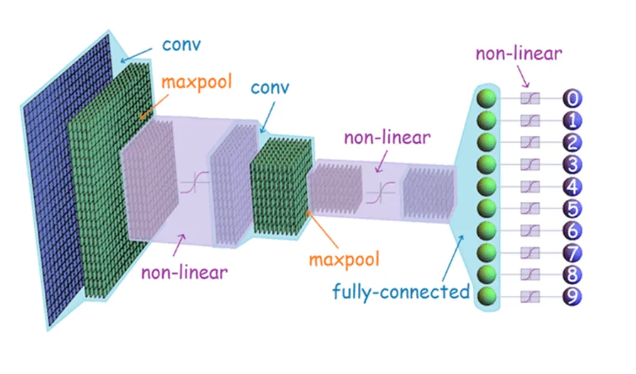
How Does a 3D Convolutional Neural Network Work?
A 3D CNN is based on the concept of convolutional neural networks (CNNs) but with the addition of a third axis, which may be temporal (as in video) or spatial (as in volumetric data).
In a traditional 2D CNN, the input consists of multiple image frames, which the network processes and analyzes. In a 3D convolutional neural network, the input includes both spatial and temporal and spatial discretisation, making it possible to analyze the relationship between frames in time.
Layers & Feature Maps
The 3D convolutional neural network architecture comprises several layers, including an input layer, multiple convolutional layers, activation functions, max-pooling layers, and a final classification layer.
The convolutional layers learn and extract spatial and temporal features from the input. Activation functions introduce non-linearity into the model, allowing it to model complex relationships between the input and the target output.
Feature maps are arrays of values representing a certain feature in an image, such as an edge or a texture. The map is generated by applying convolutional filters to an input image. The filters scan the image and detect patterns at different scales, producing maps.
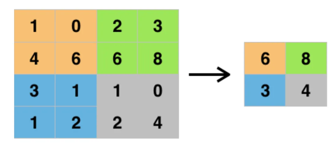
Max-Pooling Layers
“Max-pooling” reduces the size of the map by dividing it into non-overlapping regions (often squares) and taking the max value in each region. Max-pooling layers preserve important features in the map by retaining the maximum activation value within each region while reducing the size of the feature map, making the network more computationally efficient. Furthermore, reducing the feature map’s size helps the network to be more robust to small translations in the input image, as the max-pooling operation is invariant to small translations.
Fully Connected Layers
The classification layer typically comprises one or more fully connected (dense) layers connected to each neuron in the previous layer. The predictions made by the classification layer are based on the learned features from the previous layers. These features can include edges, textures, and shapes. Thus, classification layers are a crucial component of a Convolutional Neural Network to make predictions based on the features learned by the network.
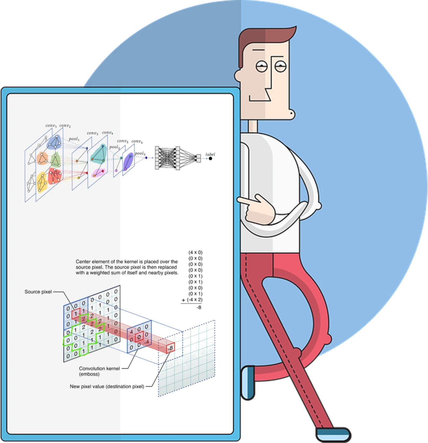
Convolution in Detail
Convolution is a mathematical operation that allows information from one function to be transformed and combined with another. It is widely used in image processing, signal processing, and ML. Convolution can be represented mathematically using convolutional operators, which are functions that define how the input and output channels are related.
The Mathematics of Convolution
The convolution operation between signals f and g can be mathematically expressed as
(f*g)(t) = ∫ f(τ) g(t - τ) dτ,
where f and g are input signals, t is time, ∫ signifies an integral over time (with τ as the dummy variable of integration), and ‘*’ denotes the convolution operator.
The convolution ‘*’ generates an output signal, which is a transformed version of the input signals.
Application to Image Processing
In image processing, the input signals can be viewed as pixels, and the convolutional operator functions as a filter. This filter is applied to each region of the image, producing a transformed version that highlights specific features. Repeating this process with different convolutional filters allows the extraction of various image features. Convolution in image processing and ML offers many advantages over older methods.
Advantages of Convolution
One major benefit is its capacity to automatically extract features from the input, unlike traditional techniques that required manual feature extraction, which was time-consuming and labor-intensive. Additionally, convolution preserves the spatial structure of the input because it is applied locally, considering only a small region at a time. This is crucial for tasks like object recognition and image classification.
Convolutional layers in deep networks learn to identify the most relevant features within the input. These filters are adjusted during training to optimize model performance. Lastly, convolution is computationally efficient on modern hardware, making it suitable for real-time applications.
In summary, convolution is a powerful mathematical operation that offers practical benefits in image processing through its ability to automatically extract features, maintain spatial data structure, learn patterns, and operate efficiently.
What is a gCNN?
A geodesic 3D convolutional neural network (gCNN) is a 3D convolutional neural network using geodesic instead of traditional 3D convolutions. Geodesic convolutions consider the intrinsic geometry of the processed data.
Instances are the curvature or shape of objects with bumps. gCCNs are often used in medical applications: for example, organs, bones, and tissues often have complex shapes that can be better captured and analyzed using geodesic convolutions. 3D CNNs improve diagnostic accuracy and patient outcomes by analyzing CT and MRI scans. Thus, 3D CNNs have proven useful in analyzing MRI and CT scans for diagnostic purposes.
What Are the Advantages of gCNN
The advantages are twofold:
- Geodesic convolutions can better analyse the data's intrinsic geometry and improve the model accuracy.
- Geodesic convolutions can be more computationally efficient than traditional CNNs, as they only consider the most important information in the data. The reduced number of parameters in the model, the reduced number of computations required for each convolution operation, and the reduced amount of data to be processed all contribute to efficiency.
More on gCNNs
Traditional convolutional neural networks (CNNs) use a fixed grid structure to process the input, resulting in a loss of information about the intrinsic data geometry. On the other hand, geodesic convolutions use a flexible grid structure adapted to the data's geometry, allowing a more accurate representation of the data's intrinsic geometry. This is done by defining the grid structure in terms of geodesic distances, rather than Euclidean distances, between the data points. The geodesic distance between two points in the data can be computed using various techniques, including heat diffusion, shortest path algorithms, or curvature-aware algorithms. The choice of technique will depend on the specific task and the type of processed data.
What are Euclidean and Non-Euclidean Distances?
Euclidean and non-Euclidean distance measures refer to different distance measures used in CNNs.
- Euclidean distance measures the straight-line distance between two points in space.
- Non-Euclidean distance, on the other hand, refers to any distance measure that is not the Euclidean distance.
Euclidean distance
Euclidean distance is used in traditional convolutions.
In the context of CNNs, Euclidean distance is often used to define the distance between the filter and the input in a traditional convolution operation. In this case, the filter is moved across the input in a grid-like structure, with the distance between the filter and the input defined by the Euclidean distance between the two points.
Non-Euclidean distance
Non-Euclidean distance measures are used in geodesic convolutions to capture better the intrinsic geometry of the processed data.
In the context of CNNs, non-Euclidean distance measures can define the distance between the filter and the input in a geodesic convolution operation. In this case, the grid structure used to move the filter across the input is adapted to the intrinsic geometry of the data. The non-Euclidean distance measure defines the distance between the filter and the input.
Cat Example
A Euclidean manifold is a space with distance and coordinates.
In a 2D picture of a cat, pixels are points in the plane, with relationships captured by Euclidean distance, calculated as
√((x₂ - x₁)²+(y₂ - y₁)²)
Computing these distances between pixels helps in image segmentation, feature extraction, and clustering. Although pixel values are discrete, this simplified, continuous representation suffices for many image-processing tasks, enabling standard CNNs to process images effectively.
3D Convolutional Neural Network Applications
We can think of many applications for a 3D convolutional neural network, including:
- Medical Imaging
- Video Classification
- Autonomous Driving and Image Classification
- Geoscience
- Material Science
Medical Imaging
3D CNNs are powerful models for image segmentation tasks in medical imaging.
Medical imaging utilizes techniques like CT, MRI, ultrasound, and X-ray to visualize the body for diagnosis, revolutionizing medicine with non-invasive internal views. However, interpreting these images is complex and time-consuming, requiring expertise.
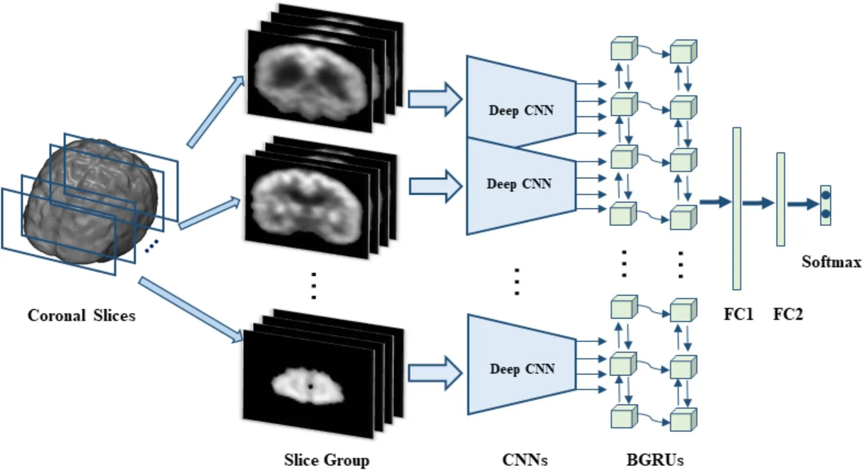
Advanced ML such as 3D CNNs can improve diagnosis accuracy and efficiency by recognizing patterns. For instance, a 3D CNN trained on MRI data could quickly identify Alzheimer's patterns and analyze multiple slices for better insights.
Video Classification
Applications of 3D CNNs in video classification include security surveillance, media entertainment, and automotive safety. These networks achieve higher accuracy by leveraging spatiotemporal features in datasets like UCF101, which focus on action recognition.
To enable this, 3D CNNs consider the entire temporal dimension of video, leading to a better understanding of visual content. This temporal modeling is key to detecting motion and recognizing actions across frames.
Training a 3D CNN model typically involves using an optimizer like Adam and an error function such as categorical cross-entropy, particularly in tasks like video classification .
Autonomous Driving and Image Classification
In autonomous driving, 3D CNNs are employed for spatiotemporal image classification tasks such as gesture recognition, pedestrian intent prediction, and vehicle behavior analysis. Unlike 2D CNNs, which process static frames independently, 3D CNNs convolve across both spatial and temporal dimensions, allowing the model to learn motion-dependent features directly from video sequences. This is critical for detecting events like sudden lane changes or braking actions, which unfold over multiple frames.
Input tensors are typically structured as (C × D × H × W), where C is the number of channels, D is the temporal depth (number of consecutive frames), and H and W are spatial dimensions.
The convolutional filters have shape (kₜ × kₕ × k_w), and the stride parameters control both spatial and temporal resolution. Temporal pooling layers reduce dimensionality while preserving motion information.
Training pipelines for image classification often use labeled video datasets like Drive&Act or HDD, capturing driver actions and scene changes. Error functions vary: categorical cross-entropy for multi-class tasks, focal loss for imbalanced classes. Optimization with Adam or RMSprop, and learning rate schedulers stabilize long sequences. Regularization techniques like dropout, jittering, and batch normalization prevent overfitting. Inference combines trained models with sensor fusion (LiDAR, radar, IMU) for real-time decisions in automotive systems.
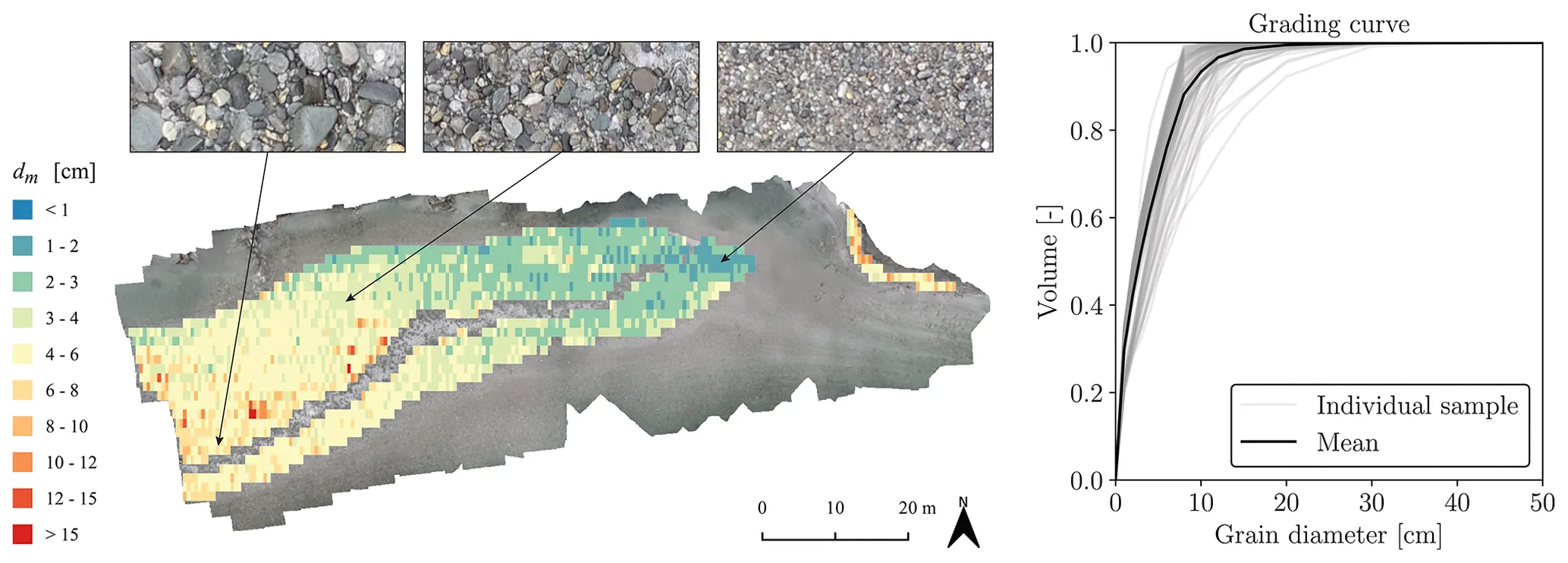
Geoscience
3D CNNs are increasingly applied in geoscience for analyzing volumetric and time-sequential data, such as seismic cubes, atmospheric simulations, and subsurface models. Capturing spatial and temporal correlations across three dimensions, 3D CNNs enable more accurate interpretation of geological structures, fault detection, and event classification. Their architecture supports input formats like (depth × height × width × time), allowing direct ingestion of raw geophysical data without extensive manual feature engineering. Training typically uses supervised learning with labeled data from well logs or historical events, optimized using error functions such as mean squared error or categorical cross-entropy, depending on the task.
Material Science
In materials science, 3D CNNs analyze volumetric imaging data such as X-ray computed tomography, electron microscopy stacks, and atomistic simulations. They learn spatial hierarchies of features from 3D structures, enabling tasks like defect detection, grain boundary segmentation, and phase classification. Input tensors represent 3D grayscale or multi-channel voxel data, with supervised training on annotated datasets. Error functions like dice coefficient or cross-entropy are used, and models benefit from GPU-accelerated training due to high data dimensionality.
3D CAD Models
Recognizing features in 3D CAD models is a critical step in automating design and manufacturing workflows, especially as traditional manufacturing transitions into smart factories.
Studying 3D CAD models is essential for the conversion of traditional manufacturing industries into smart factories. Conventional methods for recognizing machining features include graph-based, volume decomposition, hint-based, and similarity-based methods. However, the development of DL applications for machining feature recognition is motivated by the limitations of traditional methods.
FeatureNet utilizes a voxel dataset and 3D convolutional networks to recognize machining features in CAD models. Gradient-weighted class activation mapping (Grad-CAM) is applied for feature area detection in 3D CAD models using 3D CNNs.
3D CNNs have also been applied in the field of human activity recognition, video classification, and medical imaging detection, indicating their versatility beyond CAD-specific applications.
Conclusions: 3D Convolutional Neural Network Applications - 3D Simulation
- 3D CNNs Extend GNN Capabilities:
- 3D CNNs enable deep learning models to handle 3D geometrical data, extending the capabilities of graph neural networks (GNNs) to structured volumetric inputs.
- Surrogate Modeling of CAD-CAE Workflows:
- They serve as the foundation for surrogate models of numerical solvers, effectively replicating the CAD-to-CAE pipeline, including import, meshing, and solver execution.
- Origins of Neural Concept Technology:
- The Neural Concept technology originated in Switzerland, with earlt examples of hydrofoil optimization with neural networks to modern industrial deployment across sectors such as automotive, aerospace, electronics, and civil engineering.
- Addressing CAD-CAE Latency:
- In typical workflows, CAE results lag behind CAD due to simulation runtimes. 3D CNNs mitigate this by providing fast predictive models that reduce this latency dramatically.
- Bottom-Up Learning of Geometrical Features:
- The model learns how geometric patterns in CAD correlate with CAE outputs. It is trained offline using supervised learning to capture this mapping.
- Drastic Reduction in Evaluation Time:
- Once trained, the model performs predictions within 0.02 to 2 seconds, compared to hours for conventional CAE. This speed is due to lightweight activation functions and the fact that weight computation and hyperparameter tuning occur only once, during training.
- Deployment via Lightweight Applications:
- The trained model can be embedded into simplified front-end Apps for designers, sales engineers, and commissioning engineers, none of whom require simulation expertise.
- Shift from Solver-Centric to App-Centric Paradigm:
- 3D CNNs introduc a new paradigm: prepare the model once, then use it for fast, repeated execution, in contrast to classical CAE where each run is costly and slow.
- Interactive Design Space Exploration:
- Once trained, the 3D CNN enables interactive design exploration and supports integration with generative design algorithms for automated optimization.
- Proven Use Cases in Industry:
- Automotive examples include real-time aerodynamic predictions, where the surrogate model instantly provides feedback on design modifications.
- Strategic Relevance for Engineers:
- As 3D CNNs continues to influence engineering workflows, proficiency in 3D CNN concepts becomes critical for engineers aiming to remain competitive.
FAQs
What is the computational load when implementing 3D CNNs?
3D CNN implementations face computational challenges due to increased model complexity. 3D CNNs involve significantly higher computational load than 2D CNNs because they process volumetric data using 3D kernels. This leads to increased memory usage, more parameters, and longer training times. Adding more dimensions increases data and model size exponentially. Training needs high-end GPUs or distributed systems, especially for large datasets like videos or scans. Inference takes longer, limiting real-time deployment without hardware acceleration or optimization. Researchers are developing more efficient architectures and training techniques to address the challenges faced by 3D CNNs.
Why is it difficult to train 3D CNNs effectively?
3D CNNs often require large datasets for effective training, making data preparation a crucial step that can be difficult to obtain.
How can we improve the generalization ability of 3D CNNs?
Regularization techniques are essential for improving the generalization of 3D CNNs. To improve the generalization of a 3D CNN, the idea is to make the model less dependent on quirks of the training data. During training, some connections can be randomly disabled so the network cannot rely on a single pathway and must learn more robust features. The weights can also be slightly penalized when they grow too large, which discourages memorization of noise. In addition, varying the input data, by changing orientation, scaling, or cropping of volumes, forces the model to learn patterns that hold across different perspectives rather than memorizing fixed examples. Together, these techniques reduce overfitting and lead to better performance on unseen data.
How does the training time of 3D CNNs compare to that of 2D CNNs?
The training time for 3D CNNs is significantly longer than for 2D CNNs due to increased complexity.
What are the differences in performance between 3D CNN and 2D CNN for video analysis?
3D CNNs typically outperform 2D CNNs in video analysis because they capture both spatial and temporal features across consecutive frames. While 2D CNNs process each frame independently, 3D CNNs learn motion-aware patterns, which are essential for tasks like action recognition or gesture detection. However, this comes with higher computational cost and longer training times.
Are there any accuracy benchmarks available for 3D CNN?
Yes. On standard video datasets like UCF101 or Kinetics, 3D CNNs often achieve top-1 accuracy ranging from 80% to over 90%, depending on architecture depth, pretraining, and augmentation strategies. These benchmarks are commonly reported in research using models like I3D, C3D, and R(2+1)D.
What are the most common architectures used in 3D CNN?
Popular 3D CNN architectures include C3D, which uses 3×3×3 kernels throughout; I3D, which inflates 2D filters into 3D from pretrained ImageNet models; and R(2+1)D, which factorizes 3D convolutions into separate spatial and temporal operations. These are widely used in video classification and action recognition pipelines.

.webp)